2  Data Visualization

library(dplyr)
library(tidyverse)
library(gtsummary)
library(tibble)
library(ggplot2)
library(data.table)
library(DT)
library(broom)
library(devtools)
library(viridis)
library(knitr)
library(hrbrthemes)
library(car)
#using data specified in this github repository:
install_github("jhs-hwg/cardioStatsUSA")
library(cardioStatsUSA)

head(nhanes_data)

svy_id	svy_weight_mec	svy_psu	svy_strata	svy_year	svy_subpop_htn	svy_subpop_chol	demo_age_cat	demo_race	demo_race_black	demo_age_years	demo_pregnant	demo_gender	bp_sys_mean	bp_dia_mean	bp_cat_meds_excluded	bp_cat_meds_included	bp_control_jnc7	bp_control_accaha	bp_control_escesh_1	bp_control_escesh_2	bp_control_140_90	bp_control_130_80	bp_uncontrolled_jnc7	bp_uncontrolled_accaha	bp_uncontrolled_escesh_1	bp_uncontrolled_escesh_2	bp_uncontrolled_140_90	bp_uncontrolled_130_80	bp_med_use	bp_med_recommended_jnc7	bp_med_recommended_accaha	bp_med_recommended_escesh	bp_med_n_class	bp_med_n_pills	bp_med_combination	bp_med_pills_gteq_2	bp_med_ace	bp_med_aldo	bp_med_alpha	bp_med_angioten	bp_med_beta	bp_med_central	bp_med_ccb	bp_med_ccb_dh	bp_med_ccb_ndh	bp_med_diur_Ksparing	bp_med_diur_loop	bp_med_diur_thz	bp_med_renin_inhibitors	bp_med_vasod	htn_jnc7	htn_accaha	htn_escesh	htn_aware	htn_resistant_jnc7	htn_resistant_accaha	htn_resistant_jnc7_thz	htn_resistant_accaha_thz	chol_measured_never	chol_measured_last	chol_total	chol_total_gteq_200	chol_total_gteq_240	chol_hdl	chol_hdl_low	chol_trig	chol_trig_gteq_150	chol_ldl	chol_ldl_5cat	chol_ldl_lt_70	chol_ldl_gteq_70	chol_ldl_lt_100	chol_ldl_gteq_100	chol_ldl_gteq_190	chol_ldl_persistent	chol_nonhdl	chol_nonhdl_5cat	chol_nonhdl_lt_100	chol_nonhdl_gteq_100	chol_nonhdl_gteq_220	chol_med_use	chol_med_use_sr	chol_med_statin	chol_med_ezetimibe	chol_med_pcsk9i	chol_med_bile	chol_med_fibric_acid	chol_med_atorvastatin	chol_med_simvastatin	chol_med_rosuvastatin	chol_med_pravastatin	chol_med_pitavastatin	chol_med_fluvastatin	chol_med_lovastatin	chol_med_other	chol_med_addon_use	chol_med_addon_recommended_ahaacc	chol_med_statin_recommended_ahaacc	chol_med_recommended_ever	ascvd_risk_vh_ahaacc	cc_smoke	cc_bmi	cc_diabetes	cc_ckd	cc_acr	cc_egfr	cc_hba1c	cc_egfr_lt60	cc_acr_gteq30	cc_cvd_mi	cc_cvd_chd	cc_cvd_stroke	cc_cvd_ascvd	cc_cvd_hf	cc_cvd_any
12	95494.214	2	6	1999-2000	1	1	18 to 44	Non-Hispanic White	No	37	No	Men	176.6667	102.00000	SBP 160+ or DBP 100+ mm Hg	taking antihypertensive medications	No	No	No	No	No	No	Yes	Yes	Yes	Yes	Yes	Yes	Yes	Yes	Yes	Yes	One	One	No	No	Yes	No	No	No	No	No	No	No	No	No	No	No	No	No	Yes	Yes	Yes	Yes	No	No	No	No	Cholesterol has been measured previously	1 to 5 years ago	156	No	No	38	Yes	146	No	90.87551	70 to <100 mg/dL	No	Yes	Yes	No	No	No	118	100 to <130 mg/dL	No	Yes	No	No	No	No	No	No	No	No	No	No	No	No	No	No	No	No	No	No	No	No	No	Never	30 to <35	No	Yes	34.646465	83.19409	5.2	No	Yes	No	No	No	No	No	No
21	2910.630	2	3	1999-2000	1	1	18 to 44	Hispanic	No	18	No	Men	121.3333	80.00000	SBP of 130 to <140 or DBP 80 to <90 mm Hg	SBP of 130 to <140 or DBP 80 to <90 mm Hg	Yes	No	Yes	No	Yes	No	No	Yes	No	Yes	No	Yes	No	No	No	No	None	None	No	No	No	No	No	No	No	No	No	No	No	No	No	No	No	No	No	Yes	No	No	No	No	No	No	Cholesterol has been measured previously	NA	161	No	No	34	Yes	120	No	104.23559	100 to <130 mg/dL	No	Yes	No	Yes	No	No	127	100 to <130 mg/dL	No	Yes	No	No	No	No	No	No	No	No	No	No	No	No	No	No	No	No	No	No	No	No	No	NA	35+	No	No	1.600000	117.88244	5.0	No	No	NA	NA	NA	No	NA	No
27	1935.098	2	13	1999-2000	1	0	18 to 44	Hispanic	No	18	No	Men	118.0000	78.00000	SBP <120 and DBP <80 mm Hg	SBP <120 and DBP <80 mm Hg	Yes	Yes	Yes	Yes	Yes	Yes	No	No	No	No	No	No	No	No	No	No	None	None	No	No	No	No	No	No	No	No	No	No	No	No	No	No	No	No	No	No	No	No	No	No	No	No	NA	NA	NA	NA	NA	NA	NA	NA	NA	NA	NA	NA	NA	NA	NA	NA	NA	NA	NA	NA	NA	NA	NA	NA	NA	NA	NA	NA	NA	NA	NA	NA	NA	NA	NA	NA	NA	NA	NA	NA	NA	NA	NA	25 to <30	No	No	4.800000	NA	NA	NA	No	NA	NA	NA	No	NA	No
28	41107.191	2	1	1999-2000	1	1	18 to 44	Non-Hispanic White	No	18	No	Men	94.0000	42.66667	SBP <120 and DBP <80 mm Hg	SBP <120 and DBP <80 mm Hg	Yes	Yes	Yes	Yes	Yes	Yes	No	No	No	No	No	No	No	No	No	No	None	None	No	No	No	No	No	No	No	No	No	No	No	No	No	No	No	No	No	No	No	No	No	No	No	No	Cholesterol has been measured previously	NA	151	No	No	64	No	52	No	75.74248	70 to <100 mg/dL	No	Yes	Yes	No	No	No	87	< 100 mg/dL	Yes	No	No	No	No	No	No	No	No	No	No	No	No	No	No	No	No	No	No	No	No	No	No	NA	<25	No	No	13.127572	139.84511	4.8	No	No	NA	NA	NA	No	NA	No
56	89768.526	1	12	1999-2000	1	0	18 to 44	Non-Hispanic White	No	21	No	Men	121.0000	65.00000	SBP of 120 to <130 and DBP <80 mm Hg	SBP of 120 to <130 and DBP < 80 mm Hg	Yes	Yes	Yes	Yes	Yes	Yes	No	No	No	No	No	No	No	No	No	No	None	None	No	No	No	No	No	No	No	No	No	No	No	No	No	No	No	No	No	No	No	No	No	No	No	No	NA	NA	NA	NA	NA	NA	NA	NA	NA	NA	NA	NA	NA	NA	NA	NA	NA	NA	NA	NA	NA	NA	NA	NA	NA	NA	NA	NA	NA	NA	NA	NA	NA	NA	NA	NA	NA	NA	NA	NA	NA	NA	Former	<25	No	No	2.715232	126.51034	5.5	No	No	No	No	No	No	No	No
57	102609.750	2	5	1999-2000	1	1	18 to 44	Non-Hispanic White	No	39	No	Men	119.3333	85.33333	SBP of 130 to <140 or DBP 80 to <90 mm Hg	SBP of 130 to <140 or DBP 80 to <90 mm Hg	Yes	No	Yes	No	Yes	No	No	Yes	No	Yes	No	Yes	No	No	No	No	None	None	No	No	No	No	No	No	No	No	No	No	No	No	No	No	No	No	No	Yes	No	Yes	No	No	No	No	Cholesterol has been measured previously	>5 years ago (possibly never)	243	Yes	Yes	46	Yes	97	No	179.25406	130 to <190 mg/dL	No	Yes	No	Yes	No	No	197	160 to <220 mg/dL	No	Yes	No	No	No	No	No	No	No	No	No	No	No	No	No	No	No	No	No	No	No	No	No	Never	25 to <30	No	No	1.028807	91.68801	4.9	No	No	No	No	No	No	No	No

print(nrow(nhanes_data))

[1] 59799

print(nrow(nhanes_data[svy_subpop_htn == 1]))

[1] 56017

2.1 Descriptive Graphs

2.1.1 Demographic Histograms (Blood Pressure vs Demographic Variables)

Systolic vs Age and Systolic vs Gender are very clear

nhanes_data %>% drop_na(bp_dia_mean) %>%
  ggplot(aes(x=bp_dia_mean, color=demo_age_cat)) +
    geom_histogram(fill="white", alpha=0.5, bins = 80) +
    ggtitle("Blood Pressure (Diastolic) with Age")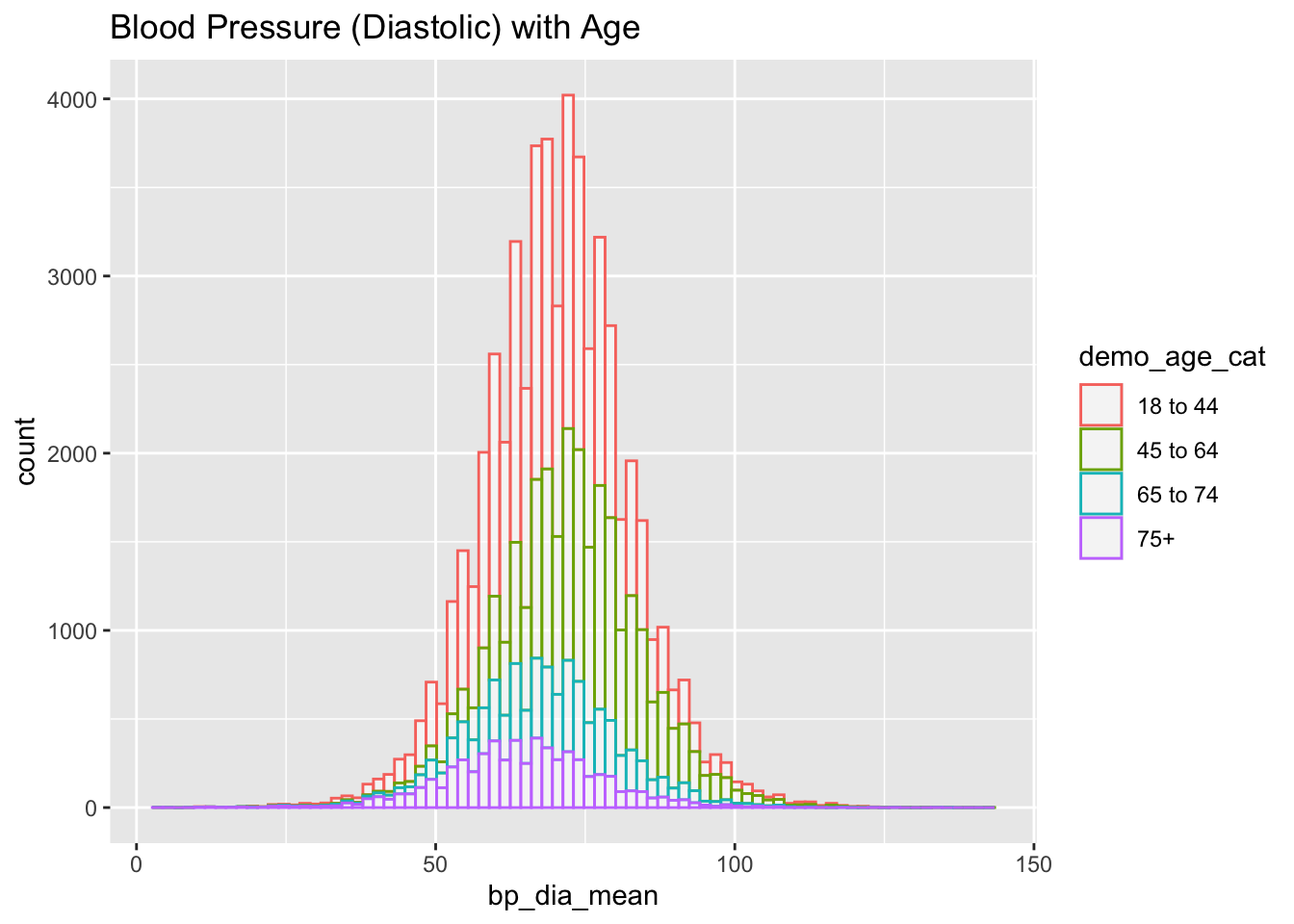

nhanes_data %>% drop_na(bp_sys_mean) %>%
  ggplot(aes(x=bp_sys_mean, color=demo_age_cat)) +
    geom_histogram(fill="white", alpha=0.5, bins = 80) +
    ggtitle("Blood Pressure (Systolic) with Age")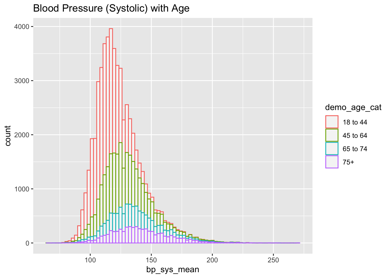

nhanes_data %>% drop_na(bp_sys_mean) %>%
  ggplot(aes(x=bp_sys_mean, color=demo_race)) +
    geom_histogram(fill="white", alpha=0.5, bins = 80) +
    ggtitle("Blood Pressure (Systolic) with Race")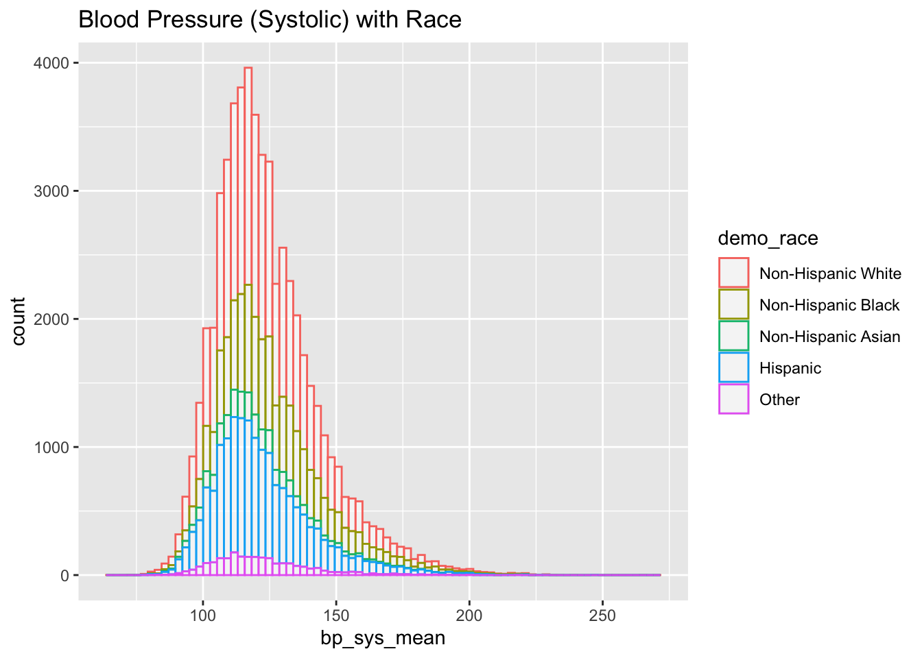

nhanes_data %>% drop_na(bp_sys_mean) %>%
  ggplot(aes(x=bp_sys_mean, color=demo_gender)) +
    geom_histogram(fill="white", alpha=0.5, bins = 80) +
    ggtitle("Blood Pressure (Systolic) with Gender")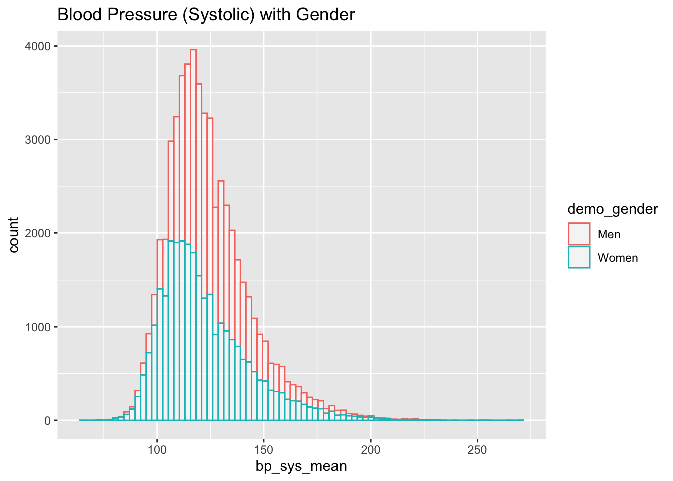

nhanes_female <- nhanes_data[nhanes_data$demo_gender == "Women", ]
nhanes_female %>% drop_na(demo_pregnant) %>% 
    ggplot(aes(x=bp_sys_mean, color=demo_pregnant)) +
    geom_histogram(fill="white", alpha=0.5, bins = 80) +
    ggtitle("Blood Pressure (Systolic) with Pregnancy (Men Excluded)")

Warning: Removed 1678 rows containing non-finite outside the scale range
(`stat_bin()`).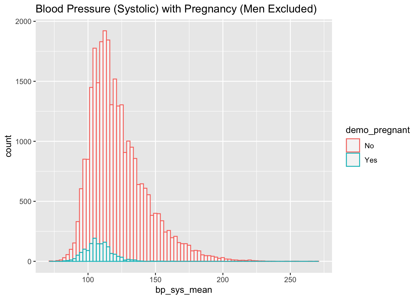

nhanes_female %>% drop_na(demo_pregnant) %>% 
    ggplot(aes(x=bp_dia_mean, color=demo_pregnant)) +
    geom_histogram(fill="white", alpha=0.5, bins = 80) +
    ggtitle("Blood Pressure (Diastolic) with Pregnancy (Men Excluded)")

Warning: Removed 1809 rows containing non-finite outside the scale range
(`stat_bin()`).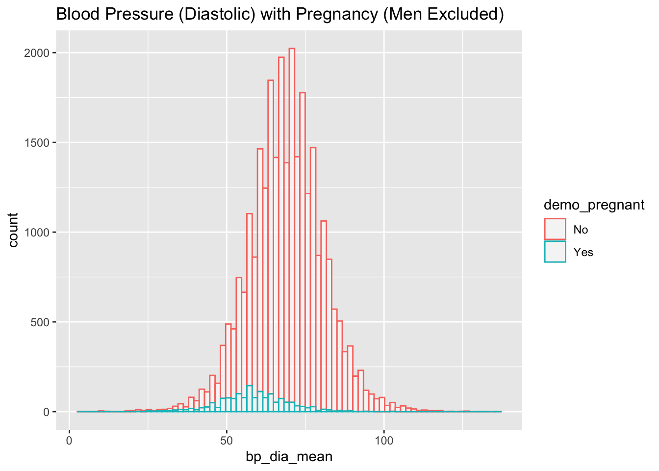

2.1.2 Comorbidities Box Plots (Blood Pressure vs Covariate)

nhanes_data %>% drop_na(cc_smoke) %>%
  ggplot(aes(x=cc_smoke, y=bp_sys_mean, fill=cc_smoke)) +
    geom_boxplot() +
    scale_fill_viridis(discrete = TRUE, alpha=0.6) +
    theme_ipsum() +
    theme(
      legend.position="none",
      plot.title = element_text(size=11)
    ) +
    ggtitle("Blood Pressure VS Smoking Status") +
    xlab("")

Warning: Removed 3111 rows containing non-finite outside the scale range
(`stat_boxplot()`).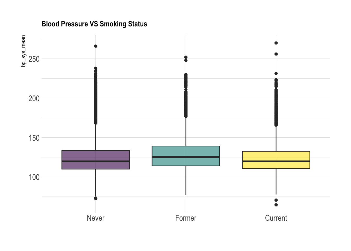

nhanes_data %>% drop_na(cc_bmi) %>%
  ggplot(aes(x=cc_bmi, y=bp_sys_mean, fill=cc_bmi)) +
    geom_boxplot() +
    scale_fill_viridis(discrete = TRUE, alpha=0.6) +
    theme_ipsum() +
    theme(
      legend.position="none",
      plot.title = element_text(size=11)
    ) +
    ggtitle("Blood Pressure VS BMI Status") +
    xlab("")

Warning: Removed 2867 rows containing non-finite outside the scale range
(`stat_boxplot()`).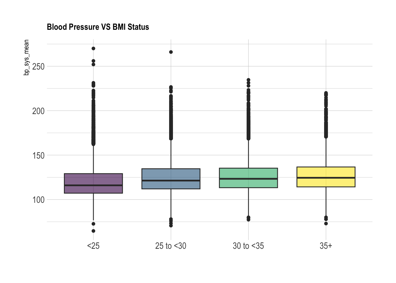

nhanes_data %>% drop_na(cc_cvd_chd) %>%
  ggplot(aes(x=cc_cvd_chd, y=bp_sys_mean, fill=cc_cvd_chd)) +
    geom_boxplot() +
    scale_fill_viridis(discrete = TRUE, alpha=0.6) +
    theme_ipsum() +
    theme(
      legend.position="none",
      plot.title = element_text(size=11)
    ) +
    ggtitle("Blood Pressure VS Chronic Heart Disease Status") +
    xlab("")

Warning: Removed 3049 rows containing non-finite outside the scale range
(`stat_boxplot()`).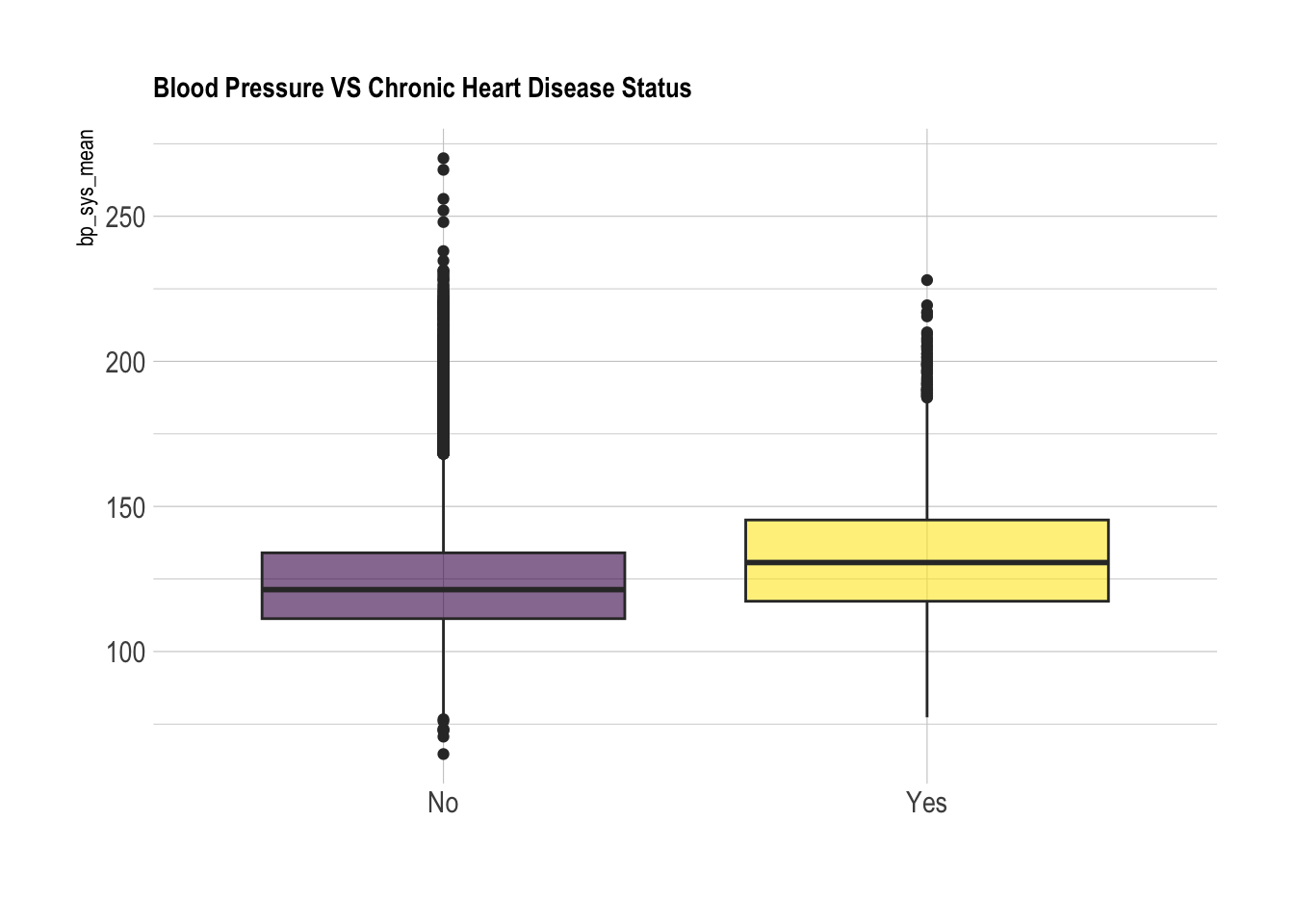

nhanes_data %>% drop_na(cc_ckd) %>%
  ggplot(aes(x=cc_ckd, y=bp_sys_mean, fill=cc_ckd)) +
    geom_boxplot() +
    scale_fill_viridis(discrete = TRUE, alpha=0.6) +
    theme_ipsum() +
    theme(
      legend.position="none",
      plot.title = element_text(size=11)
    ) +
    ggtitle("Blood Pressure VS Chronic Kidney Disease Status") +
    xlab("")

Warning: Removed 3265 rows containing non-finite outside the scale range
(`stat_boxplot()`).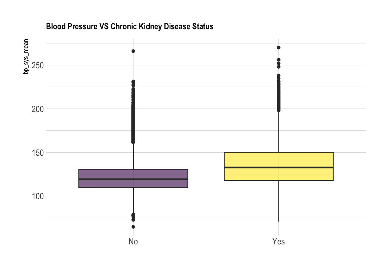

nhanes_data %>% drop_na(cc_diabetes) %>%
  ggplot(aes(x=cc_diabetes, y=bp_sys_mean, fill=cc_diabetes)) +
    geom_boxplot() +
    scale_fill_viridis(discrete = TRUE, alpha=0.6) +
    theme_ipsum() +
    theme(
      legend.position="none",
      plot.title = element_text(size=11)
    ) +
    ggtitle("Blood Pressure VS Diabetes") +
    xlab("")

Warning: Removed 3265 rows containing non-finite outside the scale range
(`stat_boxplot()`).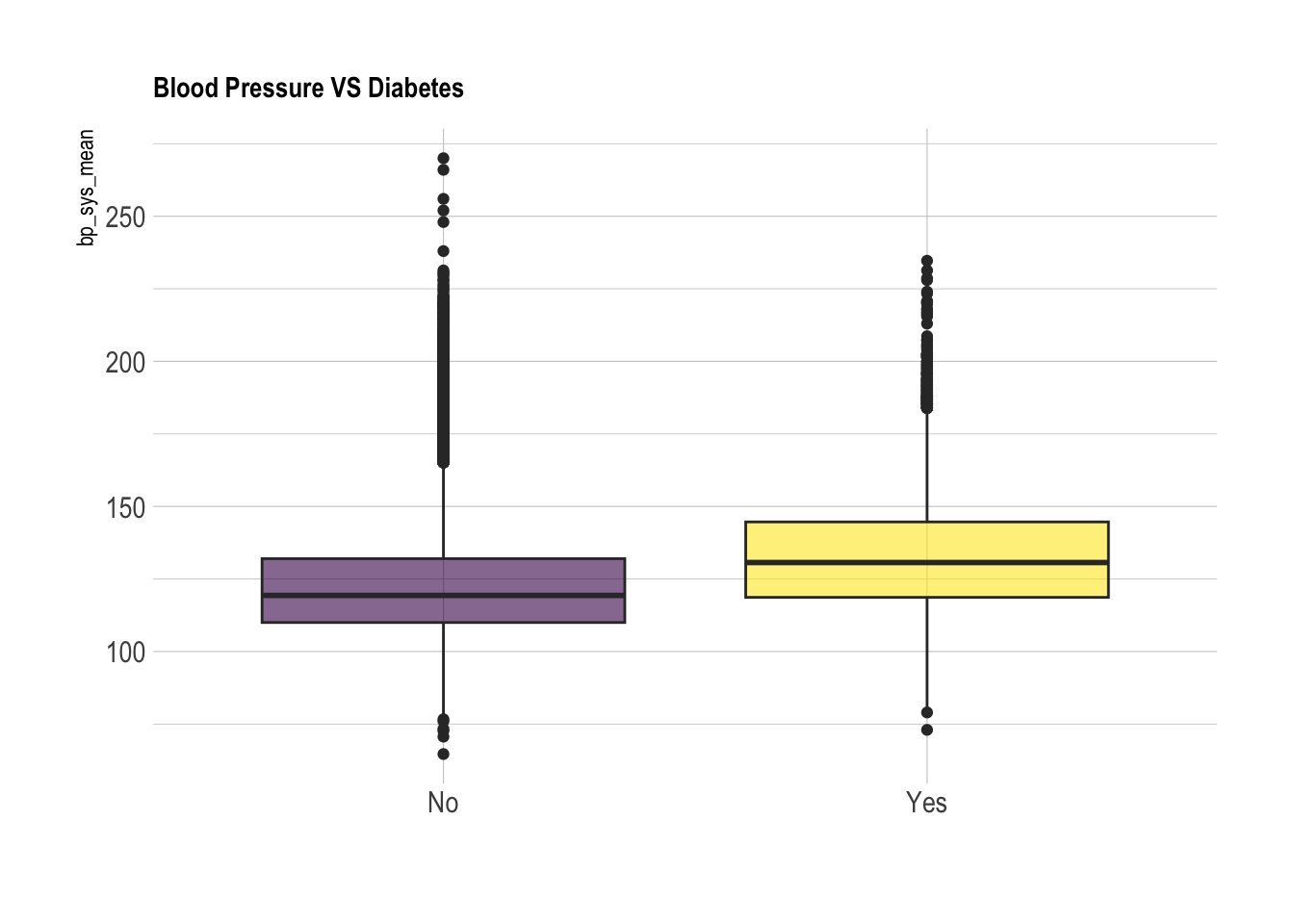

2.1.3 Comorbidities Histograms (Blood Pressure vs Covariate)

nhanes_data %>% drop_na(cc_smoke) %>%
  ggplot(aes(x=bp_sys_mean, color=cc_smoke)) +
    geom_histogram(fill="white", alpha=0.5, bins= 80) +
    scale_fill_viridis(discrete = TRUE, alpha=0.6) +
    ggtitle("Blood Pressure with Smoking Histogram")

Warning: Removed 3111 rows containing non-finite outside the scale range
(`stat_bin()`).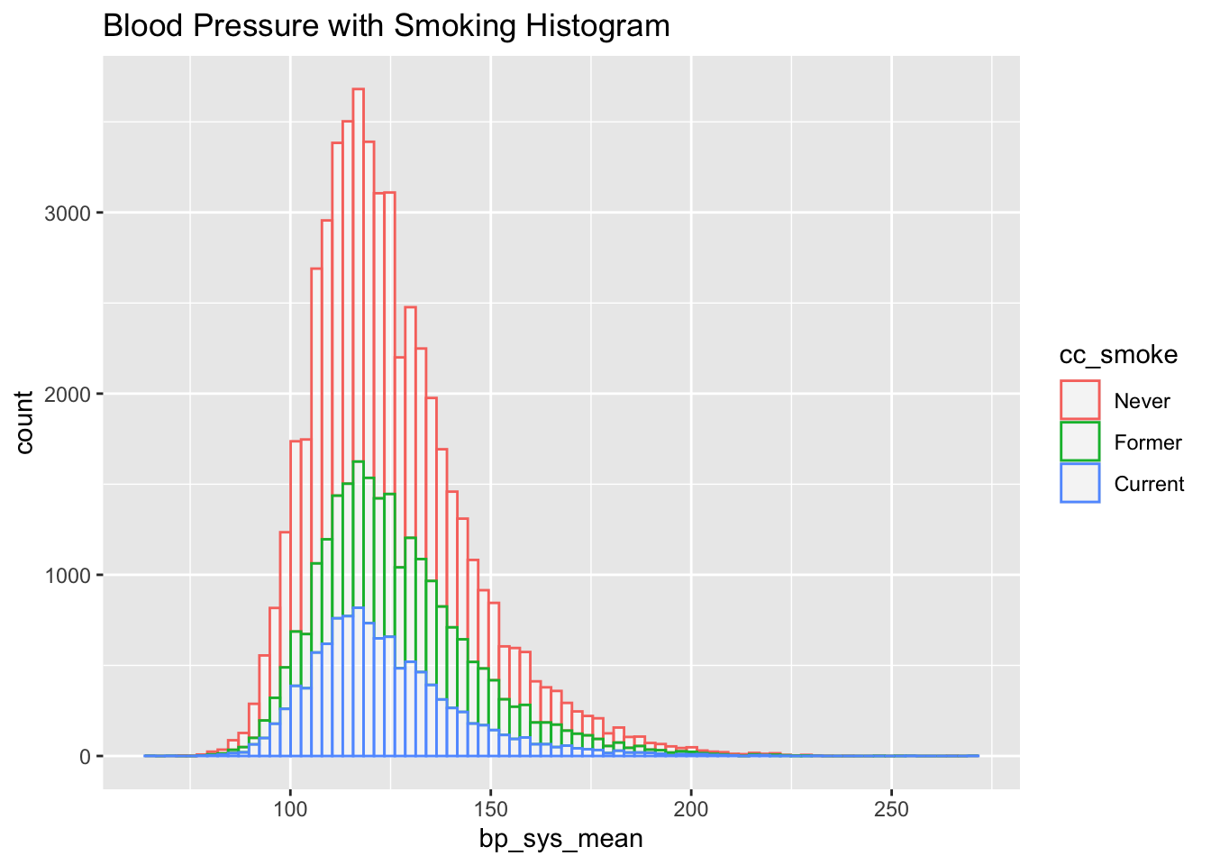

nhanes_data %>% drop_na(cc_bmi) %>%
  ggplot(aes(x=bp_sys_mean, color=cc_bmi)) +
    geom_histogram(fill="white", alpha=0.5, bins = 80) +
    ggtitle("Blood Pressure with BMI Histogram")

Warning: Removed 2867 rows containing non-finite outside the scale range
(`stat_bin()`).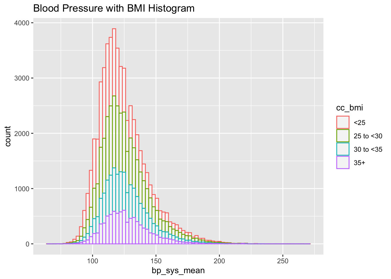

nhanes_data %>% drop_na(cc_cvd_stroke) %>%
  ggplot(aes(x=bp_sys_mean, color=cc_cvd_stroke)) +
    geom_histogram(fill="white", alpha=0.5, bins = 80) +
    ggtitle("Blood Pressure with Stroke Histogram")

Warning: Removed 3050 rows containing non-finite outside the scale range
(`stat_bin()`).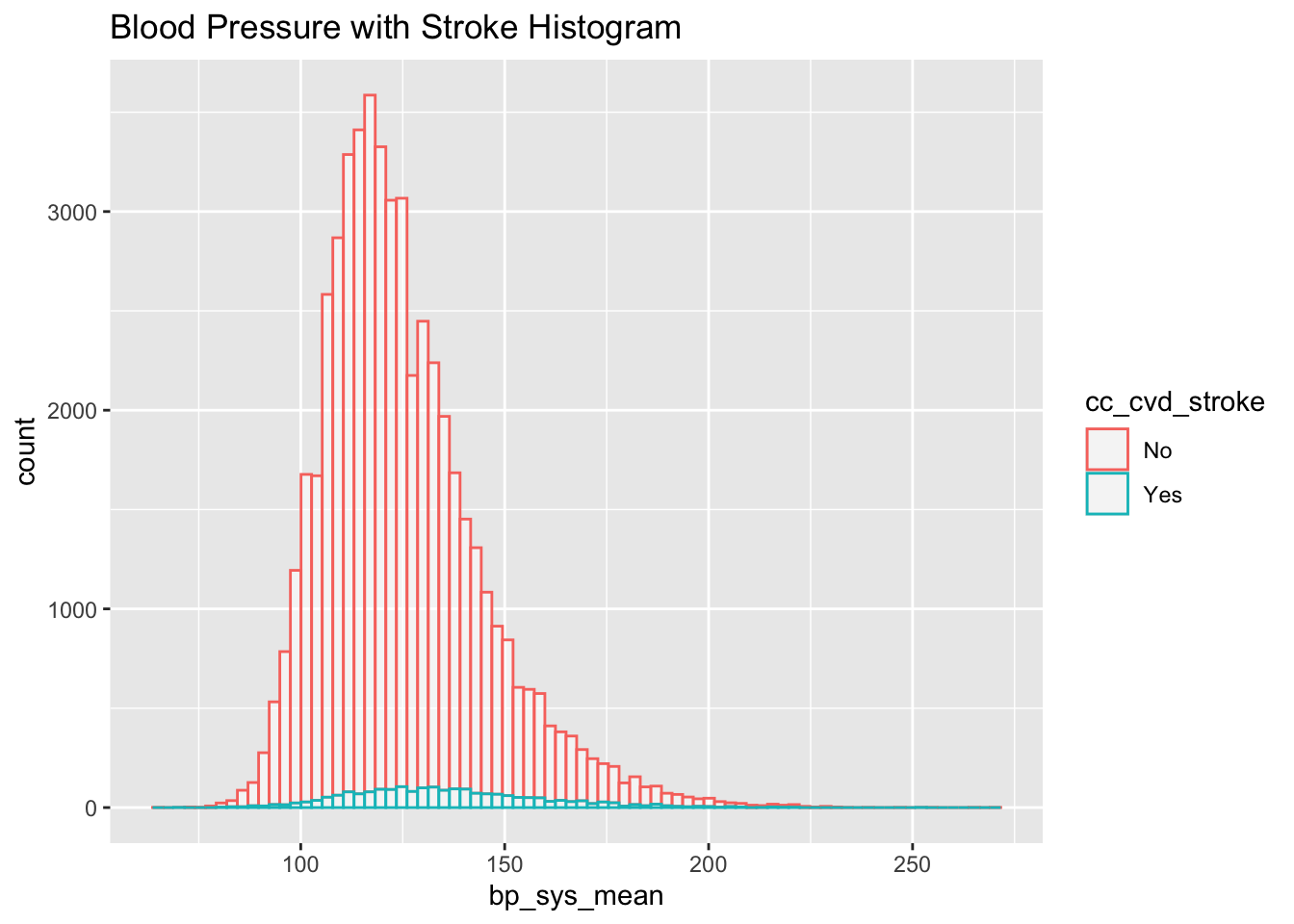

nhanes_data %>% drop_na(cc_diabetes) %>%
  ggplot(aes(x=bp_sys_mean, color=cc_diabetes)) +
    geom_histogram(fill="white", alpha=0.5, bins = 80) +
    ggtitle("Blood Pressure with Diabetes Histogram")

Warning: Removed 3265 rows containing non-finite outside the scale range
(`stat_bin()`).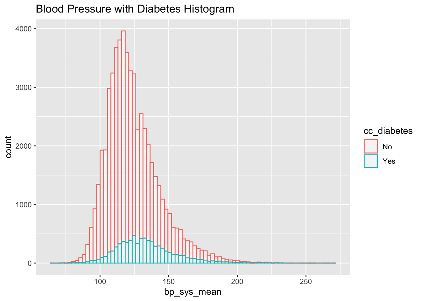

2.1.4 Chi Squared Tests (Testing difference between covariates and hypertension status)

I realize this isn’t very useful (of course the result will be significant) but I left them in anyways

#Body Mass Index
nhanes_bmi_df <- nhanes_data %>% select(htn_accaha, cc_bmi) %>% drop_na(cc_bmi)
nhanes_bmi_df <- table(nhanes_bmi_df$htn_accaha, nhanes_bmi_df$cc_bmi)
chisq.test(nhanes_bmi_df)

    Pearson's Chi-squared test

data:  nhanes_bmi_df
X-squared = 2576, df = 3, p-value < 2.2e-16

#Smoking 
nhanes_smoke_df <- nhanes_data %>% select(htn_accaha, cc_smoke) %>% drop_na(cc_smoke)
nhanes_smoke_df <- table(nhanes_smoke_df$htn_accaha, nhanes_smoke_df$cc_smoke)
chisq.test(nhanes_smoke_df)

    Pearson's Chi-squared test

data:  nhanes_smoke_df
X-squared = 991.83, df = 2, p-value < 2.2e-16

#Chronic Heart Disease
nhanes_chd_df <- nhanes_data %>% select(htn_accaha, cc_cvd_chd) %>% drop_na(cc_cvd_chd)
nhanes_chd_df <- table(nhanes_chd_df$htn_accaha, nhanes_chd_df$cc_cvd_chd)
chisq.test(nhanes_chd_df)

    Pearson's Chi-squared test with Yates' continuity correction

data:  nhanes_chd_df
X-squared = 1357.9, df = 1, p-value < 2.2e-16

#Chronic Kidney Disease
nhanes_ckd_df <- nhanes_data %>% select(htn_accaha, cc_ckd) %>% drop_na(cc_ckd)
nhanes_ckd_df <- table(nhanes_ckd_df$htn_accaha, nhanes_ckd_df$cc_ckd)
chisq.test(nhanes_ckd_df)

    Pearson's Chi-squared test with Yates' continuity correction

data:  nhanes_ckd_df
X-squared = 3702.1, df = 1, p-value < 2.2e-16

2.1.5 Two Sample T Tests

(Testing the Difference in blood pressure between comorbidities)

Should I extend to demographic data?

#Don't know if this is the idea but:
nhanes_dia_df <- nhanes_data %>% select(htn_accaha, bp_dia_mean) %>% drop_na(bp_dia_mean)
t_test <- t.test(bp_dia_mean ~ htn_accaha, data=nhanes_dia_df)
t_test

    Welch Two Sample t-test

data:  bp_dia_mean by htn_accaha
t = -96.487, df = 45747, p-value < 2.2e-16
alternative hypothesis: true difference in means between group No and group Yes is not equal to 0
95 percent confidence interval:
 -9.443644 -9.067610
sample estimates:
 mean in group No mean in group Yes 
         65.87311          75.12873 

#Smoking T Test (Excludes Former):
nhanes_sys_smoke <- nhanes_data[nhanes_data$cc_smoke != "Former", ] %>% select(cc_smoke, bp_sys_mean) %>% drop_na(bp_sys_mean) %>% drop_na(cc_smoke)
smoke_test <- t.test(bp_sys_mean ~ cc_smoke, data = nhanes_sys_smoke)
smoke_test

    Welch Two Sample t-test

data:  bp_sys_mean by cc_smoke
t = 0.85479, df = 20379, p-value = 0.3927
alternative hypothesis: true difference in means between group Never and group Current is not equal to 0
95 percent confidence interval:
 -0.2343734  0.5968840
sample estimates:
  mean in group Never mean in group Current 
             123.6788              123.4975 

#BMI T Test (Compares <25 and 35+):
nhanes_sys_bmi <- nhanes_data[nhanes_data$cc_bmi %in% c("<25", "35+"), ] %>% select(cc_bmi, bp_sys_mean) %>% drop_na(bp_sys_mean) %>% drop_na(cc_bmi)
bmi_test <- t.test(bp_sys_mean ~ cc_bmi, data = nhanes_sys_bmi)
bmi_test

    Welch Two Sample t-test

data:  bp_sys_mean by cc_bmi
t = -26.614, df = 18857, p-value < 2.2e-16
alternative hypothesis: true difference in means between group <25 and group 35+ is not equal to 0
95 percent confidence interval:
 -6.963786 -6.008393
sample estimates:
mean in group <25 mean in group 35+ 
          120.332           126.818 

#Diabetes T Test:
nhanes_sys_diabetes <- nhanes_data %>% select(cc_diabetes, bp_sys_mean) %>% drop_na(bp_sys_mean) %>% drop_na(cc_diabetes)
diabetes_test <- t.test(bp_sys_mean ~ cc_diabetes, data = nhanes_sys_diabetes)
diabetes_test

    Welch Two Sample t-test

data:  bp_sys_mean by cc_diabetes
t = -40.314, df = 9221.3, p-value < 2.2e-16
alternative hypothesis: true difference in means between group No and group Yes is not equal to 0
95 percent confidence interval:
 -10.84351  -9.83791
sample estimates:
 mean in group No mean in group Yes 
         122.7845          133.1252 

2.2 Simple Diabetes Modeling

We are choosing Diabetes as the co-morbidity for modeling. We will try to predict the occurrence of diabetes as a function of blood pressure as well as other covariates.

The most basic model possible is a simple logistic regression model predicting diabetes status based on blood pressure:

simple_diab_model_sys <- glm(cc_diabetes ~ bp_sys_mean, data = nhanes_data, family = binomial)

summary(simple_diab_model_sys)

Call:
glm(formula = cc_diabetes ~ bp_sys_mean, family = binomial, data = nhanes_data)

Coefficients:
              Estimate Std. Error z value Pr(>|z|)    
(Intercept) -4.9404827  0.0770324  -64.14   <2e-16 ***
bp_sys_mean  0.0238141  0.0005811   40.98   <2e-16 ***
---
Signif. codes:  0 '***' 0.001 '**' 0.01 '*' 0.05 '.' 0.1 ' ' 1

(Dispersion parameter for binomial family taken to be 1)

    Null deviance: 43614  on 56533  degrees of freedom
Residual deviance: 41987  on 56532  degrees of freedom
  (3265 observations deleted due to missingness)
AIC: 41991

Number of Fisher Scoring iterations: 4

knitr::kable(tidy(simple_diab_model_sys, exponentiate = TRUE, conf.int = TRUE))

term	estimate	std.error	statistic	p.value	conf.low	conf.high
(Intercept)	0.0071511	0.0770324	-64.13512	0	0.0061477	0.0083151
bp_sys_mean	1.0240999	0.0005811	40.98151	0	1.0229344	1.0252673

simple_diab_model_dia <- glm(cc_diabetes ~ bp_dia_mean, data = nhanes_data, family = binomial)

summary(simple_diab_model_dia)

Call:
glm(formula = cc_diabetes ~ bp_dia_mean, family = binomial, data = nhanes_data)

Coefficients:
             Estimate Std. Error z value Pr(>|z|)    
(Intercept) -1.652673   0.073728 -22.416  < 2e-16 ***
bp_dia_mean -0.003651   0.001039  -3.514 0.000441 ***
---
Signif. codes:  0 '***' 0.001 '**' 0.01 '*' 0.05 '.' 0.1 ' ' 1

(Dispersion parameter for binomial family taken to be 1)

    Null deviance: 43309  on 56285  degrees of freedom
Residual deviance: 43297  on 56284  degrees of freedom
  (3513 observations deleted due to missingness)
AIC: 43301

Number of Fisher Scoring iterations: 4

knitr::kable(tidy(simple_diab_model_dia, exponentiate = TRUE, conf.int = TRUE))

term	estimate	std.error	statistic	p.value	conf.low	conf.high
(Intercept)	0.1915372	0.0737285	-22.415661	0.0000000	0.1657332	0.2212722
bp_dia_mean	0.9963553	0.0010390	-3.514294	0.0004409	0.9943280	0.9983860

2.2.0.1 Model Explanation:

For the logistic regression using systolic blood pressure, we can see that the odds ratio beta parameter is 1.024. This implies that a higher systolic blood pressure corresponds to increased chances of observing diabetes.

A more exact interpretation would be that: for one additional unit increase in systolic blood pressure, the estimated risk of having diabetes increases by 2.4%.

This value may not seem extremely high, yet it still has a p value evaluated to be 0 by R. We can also see that the 95% confidence interval of this parameter ranges between 1.0229 and 1.0253, meaning that the model predicts that the true relationship falls within this interval with a 95% certainty, since the true value of the parameter is most likely within this interval.

The opposite is true with diastolic blood pressure: the beta parameter is 0.996, implying that higher diastolic blood pressure corresponds to a lower chance of observing diabetes. For an additional unit increase in diastolic blood pressure, the estimated risk of having diabetes decreases by 0.04%.

Note: systolic blood pressure is a better predictor of cardiovascular disease, so I chose to consider systolic rather than diastolic in future models.

2.3 Demographic Model

Next, we build a model including the demographic variables as well. This will hopefully provide a more accurate model, since it will have access to the further information in order to make predictions.

demo_diab_model_sys <- glm(cc_diabetes ~ bp_sys_mean + demo_age_years + demo_race + demo_gender,data = nhanes_data, family = binomial)

summary (demo_diab_model_sys)

Call:
glm(formula = cc_diabetes ~ bp_sys_mean + demo_age_years + demo_race + 
    demo_gender, family = binomial, data = nhanes_data)

Coefficients:
                              Estimate Std. Error z value Pr(>|z|)    
(Intercept)                 -5.6927561  0.0885174 -64.312  < 2e-16 ***
bp_sys_mean                  0.0037581  0.0006792   5.533 3.14e-08 ***
demo_age_years               0.0529545  0.0009161  57.806  < 2e-16 ***
demo_raceNon-Hispanic Black  0.9034242  0.0350353  25.786  < 2e-16 ***
demo_raceNon-Hispanic Asian  0.8093210  0.0606852  13.336  < 2e-16 ***
demo_raceHispanic            0.8592775  0.0343392  25.023  < 2e-16 ***
demo_raceOther               0.7478892  0.0718834  10.404  < 2e-16 ***
demo_genderWomen            -0.1547613  0.0265581  -5.827 5.63e-09 ***
---
Signif. codes:  0 '***' 0.001 '**' 0.01 '*' 0.05 '.' 0.1 ' ' 1

(Dispersion parameter for binomial family taken to be 1)

    Null deviance: 43614  on 56533  degrees of freedom
Residual deviance: 37780  on 56526  degrees of freedom
  (3265 observations deleted due to missingness)
AIC: 37796

Number of Fisher Scoring iterations: 5

knitr::kable(tidy(demo_diab_model_sys, exponentiate = TRUE, conf.int = TRUE))

term	estimate	std.error	statistic	p.value	conf.low	conf.high
(Intercept)	0.0033703	0.0885174	-64.312318	0	0.0028326	0.0040077
bp_sys_mean	1.0037652	0.0006792	5.533450	0	1.0024283	1.0051008
demo_age_years	1.0543817	0.0009161	57.805744	0	1.0524962	1.0562830
demo_raceNon-Hispanic Black	2.4680396	0.0350353	25.786107	0	2.3042427	2.6434926
demo_raceNon-Hispanic Asian	2.2463822	0.0606852	13.336382	0	1.9925692	2.5278493
demo_raceHispanic	2.3614540	0.0343392	25.023206	0	2.2077734	2.5259187
demo_raceOther	2.1125361	0.0718834	10.404206	0	1.8320999	2.4286788
demo_genderWomen	0.8566196	0.0265581	-5.827267	0	0.8131556	0.9023806

2.3.0.1 Model Explanation

In this model, we can still see a slight upwards trend with systolic blood pressure, although it is a bit weaker (1.024 > 1.003). With this parameter, the estimated risk of having diabetes increases only by 0.3%. Although the effect is smaller, we can see that the confidence interval is between 1.0024 and 1.0051, which does not include 1. So, although small, the positive relationship is most likely significant.

2.3.0.2 Demographics

Age:

The model also tells us that age is positively correlated with the observation of diabetes. With a log odds ratio of 1.054, it seems that every year increases the risk of diabetes occurrence by 5.4%.

Race:

The log odds ratio for categorical variables compares the other variables to the baseline “reference group”. Here, the “reference group” for the race variable is Non-Hispanic White. We can see that, in comparison to this group, all other races have significantly higher risk of diabetes: for example, the Hispanic population’s risk of diabetes occurrence is 2.36 times higher than the Non-Hispanic White population.

Gender:

With this variable, the reference group is men. We can see that women have a lower odds of having diabetes compared to men. Specifically, the risk of diabetes in women is about 85.6% of in men.

2.4 Full Model

Lastly, we want to create a model including confounding variables. To achieve this, we must first determine which other variables are confounding, meaning they have significant associations with diabetes.

We can achieve this by using chi squared test, which compares whether or not the observed ratios of diabetes and confounding variables matches the ratios expected by random chance. If the chi squared test determines significance, then diabetes and the other variables commonly occur together and therefore are confounding.

2.4.0.1 Perform Chi Squared Tests:

#Testing for BMI
nhanes_bmi_diab <- nhanes_data %>% select(cc_diabetes, cc_bmi) %>% drop_na(cc_bmi) %>% drop_na(cc_diabetes)
nhanes_bmi_diab <- table(nhanes_bmi_diab)
nhanes_bmi_diab

           cc_bmi
cc_diabetes   <25 25 to <30 30 to <35   35+
        No  17390     16913      9476  6965
        Yes   974      2173      2056  2274

chisq.test(nhanes_bmi_df)

    Pearson's Chi-squared test

data:  nhanes_bmi_df
X-squared = 2576, df = 3, p-value < 2.2e-16

#Testing for Smoking
nhanes_smoke_diab <- nhanes_data %>% select(cc_diabetes, cc_smoke) %>% drop_na(cc_smoke) %>% drop_na(cc_diabetes)
nhanes_smoke_diab <- table(nhanes_smoke_diab)
nhanes_smoke_diab

           cc_smoke
cc_diabetes Never Former Current
        No  27414  11107   10366
        Yes  3917   2587    1249

chisq.test(nhanes_smoke_diab)

    Pearson's Chi-squared test

data:  nhanes_smoke_diab
X-squared = 435.81, df = 2, p-value < 2.2e-16

#Testing for Hypertensive Medication use
nhanes_med_diab <- nhanes_data %>% select(cc_diabetes, bp_med_use) %>% drop_na(bp_med_use) %>% drop_na(cc_diabetes)
nhanes_med_diab <- table(nhanes_med_diab)
nhanes_med_diab

           bp_med_use
cc_diabetes    No   Yes
        No  41679 10079
        Yes  3138  4611

chisq.test(nhanes_med_diab)

    Pearson's Chi-squared test with Yates' continuity correction

data:  nhanes_med_diab
X-squared = 5807.1, df = 1, p-value < 2.2e-16

After this analysis, we can see that all three variables, BMI, Smoking, and Medication Use, are all confounding. We can include all of them in the next model, in addition to systolic blood pressure and the demographic variables:

#to prevent errors down the line, exclude the rows with na:
used_vars = c('cc_diabetes', 'bp_sys_mean', 'demo_age_years', 'demo_race', 'demo_gender', 'cc_bmi', 'cc_smoke', 'bp_med_use')
clean_nhanes <- nhanes_data[complete.cases(nhanes_data[,..used_vars]), ]

full_diab_model_sys <- glm(cc_diabetes ~ bp_sys_mean + demo_age_years + demo_race + demo_gender+ cc_bmi + cc_smoke + bp_med_use, data = clean_nhanes, family = binomial)

summary(full_diab_model_sys)

Call:
glm(formula = cc_diabetes ~ bp_sys_mean + demo_age_years + demo_race + 
    demo_gender + cc_bmi + cc_smoke + bp_med_use, family = binomial, 
    data = clean_nhanes)

Coefficients:
                              Estimate Std. Error z value Pr(>|z|)    
(Intercept)                 -6.3003463  0.1112295 -56.643  < 2e-16 ***
bp_sys_mean                  0.0017066  0.0007373   2.315   0.0206 *  
demo_age_years               0.0470354  0.0011312  41.579  < 2e-16 ***
demo_raceNon-Hispanic Black  0.6987360  0.0374745  18.646  < 2e-16 ***
demo_raceNon-Hispanic Asian  1.3022903  0.0660355  19.721  < 2e-16 ***
demo_raceHispanic            0.8889260  0.0366792  24.235  < 2e-16 ***
demo_raceOther               0.8913458  0.0763522  11.674  < 2e-16 ***
demo_genderWomen            -0.3082492  0.0295124 -10.445  < 2e-16 ***
cc_bmi25 to <30              0.5927344  0.0444524  13.334  < 2e-16 ***
cc_bmi30 to <35              1.1736075  0.0463565  25.317  < 2e-16 ***
cc_bmi35+                    1.7702868  0.0480051  36.877  < 2e-16 ***
cc_smokeFormer               0.0614704  0.0335729   1.831   0.0671 .  
cc_smokeCurrent              0.1853436  0.0403687   4.591 4.41e-06 ***
bp_med_useYes                0.9121351  0.0314064  29.043  < 2e-16 ***
---
Signif. codes:  0 '***' 0.001 '**' 0.01 '*' 0.05 '.' 0.1 ' ' 1

(Dispersion parameter for binomial family taken to be 1)

    Null deviance: 41278  on 52196  degrees of freedom
Residual deviance: 33055  on 52183  degrees of freedom
AIC: 33083

Number of Fisher Scoring iterations: 6

knitr::kable(tidy(full_diab_model_sys, exponentiate = TRUE, conf.int = TRUE))

term	estimate	std.error	statistic	p.value	conf.low	conf.high
(Intercept)	0.0018357	0.1112295	-56.642782	0.0000000	0.0014752	0.0022815
bp_sys_mean	1.0017080	0.0007373	2.314675	0.0206307	1.0002594	1.0031545
demo_age_years	1.0481591	0.0011312	41.579121	0.0000000	1.0458438	1.0504919
demo_raceNon-Hispanic Black	2.0112090	0.0374745	18.645645	0.0000000	1.8687584	2.1644762
demo_raceNon-Hispanic Asian	3.6777100	0.0660355	19.721057	0.0000000	3.2286139	4.1827136
demo_raceHispanic	2.4325157	0.0366792	24.235131	0.0000000	2.2638469	2.6139232
demo_raceOther	2.4384090	0.0763522	11.674130	0.0000000	2.0964731	2.8282006
demo_genderWomen	0.7347322	0.0295124	-10.444726	0.0000000	0.6934113	0.7784570
cc_bmi25 to <30	1.8089279	0.0444524	13.334145	0.0000000	1.6585185	1.9742572
cc_bmi30 to <35	3.2336368	0.0463565	25.316997	0.0000000	2.9536973	3.5423428
cc_bmi35+	5.8725376	0.0480051	36.877031	0.0000000	5.3470462	6.4542286
cc_smokeFormer	1.0633990	0.0335729	1.830951	0.0671079	0.9956021	1.1356446
cc_smokeCurrent	1.2036319	0.0403687	4.591266	0.0000044	1.1117990	1.3024331
bp_med_useYes	2.4896325	0.0314064	29.042966	0.0000000	2.3411270	2.6478476

2.4.0.2 Model Explanation

The previous variables in this model continue to show the same patterns, although again, the effect of systolic blood pressure is again reduced due to a lower log odds ratio. Now, the p value seems to be much higher at 0.02 (which is still significant, but much less so). The demographic variables also have much the same pattern, although Non-Hispanic Asians seem to have a much higher odds ratio than in the previous model.

2.4.0.3 Covariates

BMI:

In this variable, the baseline reference level is bmi <25. In comparison, those with higher bmi have increased risk of having diabetes, with the risk increasing the higher the bmi becomes. For example, those with bmi from 25-30 have a 1.8 times higher risk, while those with a bmi of 35+ have a 5.8 times higher risk.

Smoking:

With a baseline level of nonsmoking, former smokers may have about a 6% higher risk of diabetes. This may not be significant, however, given that the p value is only 0.067 and the odds ratio of 1 falls within the confidence interval. Current smokers, on the other hand, have about a 20% higher risk, this time with a much lower p value of 4*10^-6

Blood Pressure Medication Use:

Compared to those who do not use blood pressure medication, individuals who do have about a 2.5 times higher risk of experiencing diabetes.

2.5 Model Selection

It is possible to find an even better model by modifying which variables we include in our logistic regression model. We can achieve this using model selection, which will selectively add or subtract our explanatory variables from the model and evaluate its performance to choose the final best set of variables.

Explanation of model selection and or AIC?

2.5.0.1 Backwards Selection:

backwards = step(full_diab_model_sys)

Start:  AIC=33082.55
cc_diabetes ~ bp_sys_mean + demo_age_years + demo_race + demo_gender + 
    cc_bmi + cc_smoke + bp_med_use

                 Df Deviance   AIC
<none>                 33055 33083
- bp_sys_mean     1    33060 33086
- cc_smoke        2    33076 33100
- demo_gender     1    33164 33190
- bp_med_use      1    33909 33935
- demo_race       4    33930 33950
- cc_bmi          3    34756 34778
- demo_age_years  1    34931 34957

formula(backwards)

cc_diabetes ~ bp_sys_mean + demo_age_years + demo_race + demo_gender + 
    cc_bmi + cc_smoke + bp_med_use

It looks like the backwards selection model returned the same full model. In other words, removing variables does not improve its AIC, and therefore does not improve its performance.

2.5.0.2 Forward Selection

#start from a model without any predictors
nothing <- glm(cc_diabetes ~ 1, data = clean_nhanes, family=binomial)
summary(nothing)

Call:
glm(formula = cc_diabetes ~ 1, family = binomial, data = clean_nhanes)

Coefficients:
            Estimate Std. Error z value Pr(>|z|)    
(Intercept) -1.85919    0.01282  -145.1   <2e-16 ***
---
Signif. codes:  0 '***' 0.001 '**' 0.01 '*' 0.05 '.' 0.1 ' ' 1

(Dispersion parameter for binomial family taken to be 1)

    Null deviance: 41278  on 52196  degrees of freedom
Residual deviance: 41278  on 52196  degrees of freedom
AIC: 41280

Number of Fisher Scoring iterations: 4

forwards = step(nothing,
scope=list(lower=formula(nothing),upper=formula(full_diab_model_sys)), direction="forward")

Start:  AIC=41279.9
cc_diabetes ~ 1

                 Df Deviance   AIC
+ bp_med_use      1    37076 37080
+ demo_age_years  1    37252 37256
+ cc_bmi          3    39218 39226
+ bp_sys_mean     1    39888 39892
+ demo_race       4    40891 40901
+ cc_smoke        2    40911 40917
+ demo_gender     1    41242 41246
<none>                 41278 41280

Step:  AIC=37079.85
cc_diabetes ~ bp_med_use

                 Df Deviance   AIC
+ demo_age_years  1    35675 35681
+ cc_bmi          3    35907 35917
+ demo_race       4    36597 36609
+ bp_sys_mean     1    36788 36794
+ cc_smoke        2    36968 36976
+ demo_gender     1    37009 37015
<none>                 37076 37080

Step:  AIC=35681.48
cc_diabetes ~ bp_med_use + demo_age_years

              Df Deviance   AIC
+ cc_bmi       3    34070 34082
+ demo_race    4    34834 34848
+ demo_gender  1    35624 35632
+ bp_sys_mean  1    35654 35662
+ cc_smoke     2    35670 35680
<none>              35675 35681

Step:  AIC=34082.43
cc_diabetes ~ bp_med_use + demo_age_years + cc_bmi

              Df Deviance   AIC
+ demo_race    4    33213 33233
+ demo_gender  1    33963 33977
+ bp_sys_mean  1    34050 34064
+ cc_smoke     2    34054 34070
<none>              34070 34082

Step:  AIC=33232.52
cc_diabetes ~ bp_med_use + demo_age_years + cc_bmi + demo_race

              Df Deviance   AIC
+ demo_gender  1    33081 33103
+ cc_smoke     2    33170 33194
+ bp_sys_mean  1    33208 33230
<none>              33213 33233

Step:  AIC=33102.89
cc_diabetes ~ bp_med_use + demo_age_years + cc_bmi + demo_race + 
    demo_gender

              Df Deviance   AIC
+ cc_smoke     2    33060 33086
+ bp_sys_mean  1    33076 33100
<none>              33081 33103

Step:  AIC=33085.88
cc_diabetes ~ bp_med_use + demo_age_years + cc_bmi + demo_race + 
    demo_gender + cc_smoke

              Df Deviance   AIC
+ bp_sys_mean  1    33055 33083
<none>              33060 33086

Step:  AIC=33082.55
cc_diabetes ~ bp_med_use + demo_age_years + cc_bmi + demo_race + 
    demo_gender + cc_smoke + bp_sys_mean

The Forward Selection process again selects the full model.

bothways = step(nothing, list(lower=formula(nothing),upper=formula(full_diab_model_sys)),
direction="both",trace=0)
formula(bothways)

cc_diabetes ~ bp_med_use + demo_age_years + cc_bmi + demo_race + 
    demo_gender + cc_smoke + bp_sys_mean

The Forward-Backward algorithm also selects all of the variables

2.6 Model Diagnostics

I followed a guide online but I don’t really know what this is doing:

clean_nhanes %>% 
  mutate(comp_res = coef(full_diab_model_sys)["demo_age_years"]*demo_age_years + residuals(full_diab_model_sys, type = "working")) %>% 
  ggplot(aes(x = demo_age_years, y = comp_res)) +
  geom_point() +
  geom_smooth(color = "red", method = "lm", linetype = 2, se = F) +
  geom_smooth(se = F)

`geom_smooth()` using formula = 'y ~ x'
`geom_smooth()` using method = 'gam' and formula = 'y ~ s(x, bs = "cs")'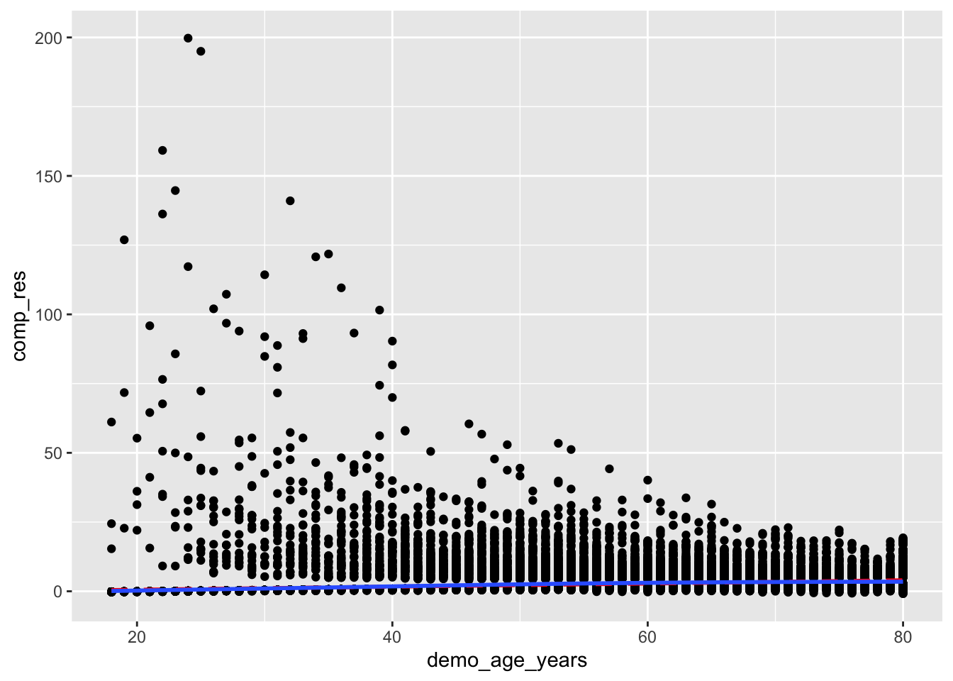

clean_nhanes %>% 
  mutate(comp_res = coef(full_diab_model_sys)["bp_sys_mean"]*bp_sys_mean + residuals(full_diab_model_sys, type = "working")) %>% 
  ggplot(aes(x = bp_sys_mean, y = comp_res)) +
  geom_point() +
  geom_smooth(color = "red", method = "lm", linetype = 2, se = F) +
  geom_smooth(se = F)

`geom_smooth()` using formula = 'y ~ x'
`geom_smooth()` using method = 'gam' and formula = 'y ~ s(x, bs = "cs")'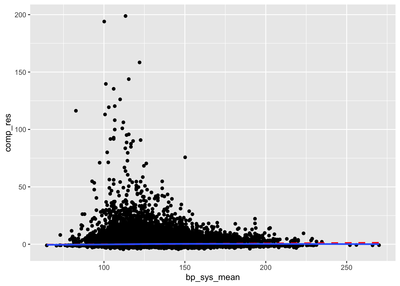

Test for Multicollinearity

vif(full_diab_model_sys)

                   GVIF Df GVIF^(1/(2*Df))
bp_sys_mean    1.169212  1        1.081301
demo_age_years 1.528167  1        1.236191
demo_race      1.207663  4        1.023866
demo_gender    1.091056  1        1.044536
cc_bmi         1.182024  3        1.028263
cc_smoke       1.173951  2        1.040908
bp_med_use     1.235766  1        1.111650

Outliers

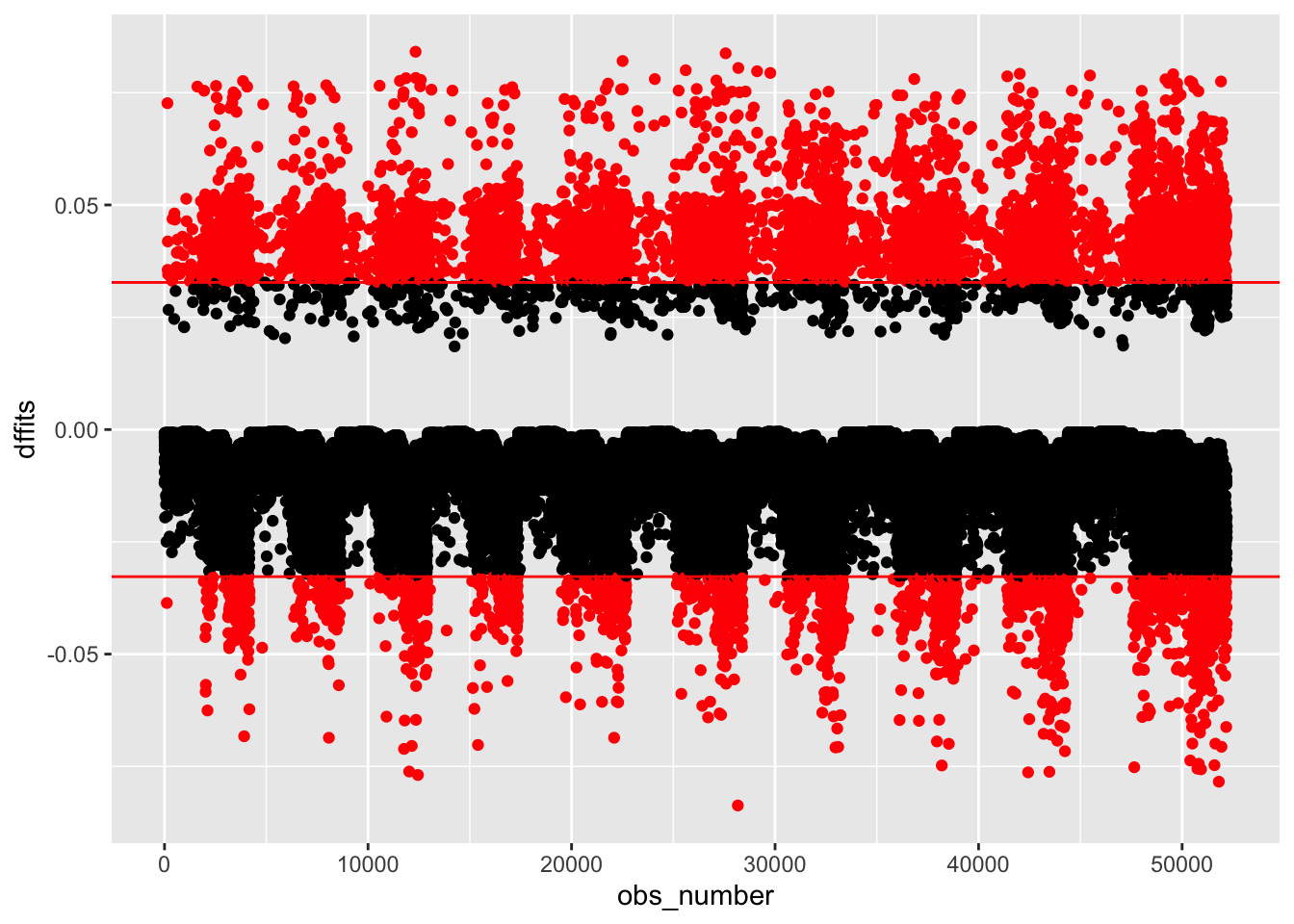
outlier_nhanes <-
  clean_nhanes %>% 
  mutate(dffits = dffits(full_diab_model_sys))

outlier_nhanes %>% 
  mutate(obs_number = row_number(),
         large = ifelse(abs(dffits) > 2*sqrt(length(coef(full_diab_model_sys))/nobs(full_diab_model_sys)),
                        "red", "black")) %>% 
  ggplot(aes(obs_number, dffits, color = large)) +
  geom_point() + 
  geom_hline(yintercept = c(-1,1) * 2*sqrt(length(coef(full_diab_model_sys))/nobs(full_diab_model_sys)), color = "red") +
  scale_color_identity()