5  Creating “Noisy” Data

library(dplyr)
library(tidyverse)
library(tibble)
library(ggplot2)
library(knitr)
library(hrbrthemes)
library(viridis)

library(devtools)
#using data specified in this github repository:
install_github("jhs-hwg/cardioStatsUSA")
library(cardioStatsUSA)

#to prevent errors, exclude the rows with na
used_vars = c('cc_diabetes', 'bp_sys_mean', 'demo_age_years', 'demo_race', 'demo_gender', 'cc_bmi', 'cc_smoke', 'bp_med_use')
clean_nhanes <- nhanes_data[complete.cases(nhanes_data[,..used_vars]), ]

In normal usage of measurement error techniques, the data is assumed to have systematic error arising from measurement of the variables which we aim to remedy. In our case, we believe that the NHANES data has no measurement error, so we will instead simulate error by adding in random noise to the existing data to create a “noisy” dataset.

First, let’s remind ourselves the relationship between blood pressure and diabetes visually:

clean_nhanes %>%
  ggplot(aes(x=bp_sys_mean, color=cc_diabetes)) +
    geom_histogram(fill="white", alpha=0.5, bins = 80) +
    ggtitle("Blood Pressure with Diabetes Histogram")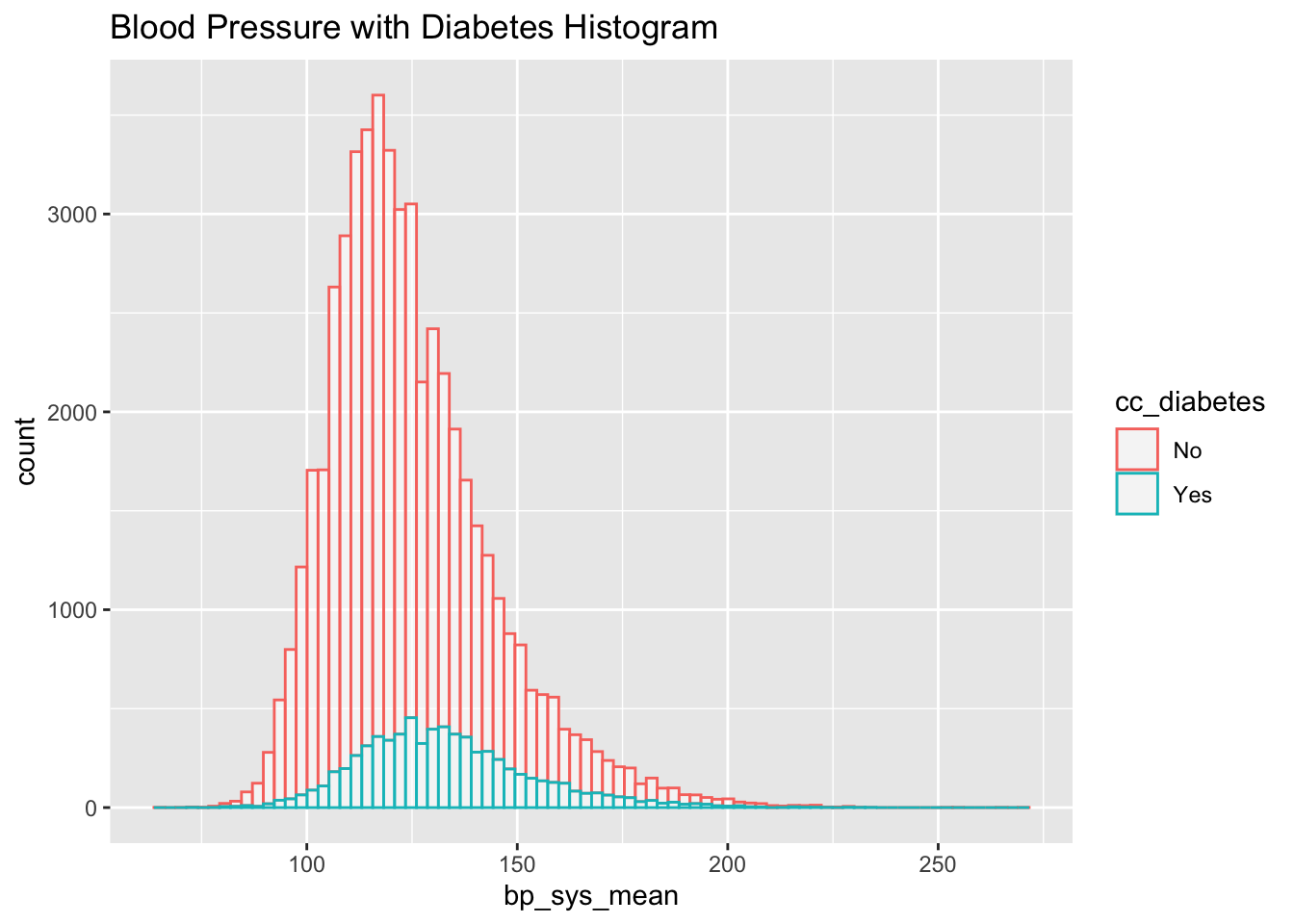

clean_nhanes %>%
  ggplot(aes(x=cc_diabetes, y=bp_sys_mean, fill=cc_diabetes)) +
    geom_boxplot() +
    scale_fill_viridis(discrete = TRUE, alpha=0.6) +
    theme_ipsum() +
    theme(
      legend.position="none",
      plot.title = element_text(size=11)
    ) +
    ggtitle("Blood Pressure VS Diabetes Status") +
    xlab("")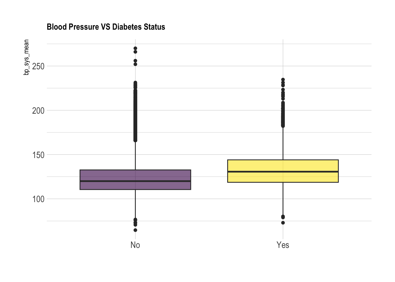

With this much data, the true true statistic (in this case, the mean blood pressure values for both groups) will be clear no matter how much noise we add. However, in normal circumstances we would not have this much data. We can instead mimic more realistic scenarios by taking a smaller subset of this data to examine. The goal will be to add noise to obscure the relationship between diabetes and blood pressure, and then use measurement error correction to rediscover the true relationship.

Let’s start by taking a subset of n=150. Since in the total data set, about 13% of individuals had diabetes, we will keep this ratio similar here.

set.seed(19)
#original: seed 52, subset yes = 20, subset no = 130

subset_diab_yes <- subset(clean_nhanes, cc_diabetes == "Yes") 
subset_diab_no <- subset(clean_nhanes, cc_diabetes == "No")

sample_diab_yes <- subset_diab_yes[sample(1:nrow(subset_diab_yes), 78, replace=FALSE),]
sample_diab_no <- subset_diab_no[sample(1:nrow(subset_diab_no), 522, replace=FALSE),]

subset_nhanes <- rbind(sample_diab_yes, sample_diab_no)
head(subset_nhanes)

svy_id	svy_weight_mec	svy_psu	svy_strata	svy_year	svy_subpop_htn	svy_subpop_chol	demo_age_cat	demo_race	demo_race_black	demo_age_years	demo_pregnant	demo_gender	bp_sys_mean	bp_dia_mean	bp_cat_meds_excluded	bp_cat_meds_included	bp_control_jnc7	bp_control_accaha	bp_control_escesh_1	bp_control_escesh_2	bp_control_140_90	bp_control_130_80	bp_uncontrolled_jnc7	bp_uncontrolled_accaha	bp_uncontrolled_escesh_1	bp_uncontrolled_escesh_2	bp_uncontrolled_140_90	bp_uncontrolled_130_80	bp_med_use	bp_med_recommended_jnc7	bp_med_recommended_accaha	bp_med_recommended_escesh	bp_med_n_class	bp_med_n_pills	bp_med_combination	bp_med_pills_gteq_2	bp_med_ace	bp_med_aldo	bp_med_alpha	bp_med_angioten	bp_med_beta	bp_med_central	bp_med_ccb	bp_med_ccb_dh	bp_med_ccb_ndh	bp_med_diur_Ksparing	bp_med_diur_loop	bp_med_diur_thz	bp_med_renin_inhibitors	bp_med_vasod	htn_jnc7	htn_accaha	htn_escesh	htn_aware	htn_resistant_jnc7	htn_resistant_accaha	htn_resistant_jnc7_thz	htn_resistant_accaha_thz	chol_measured_never	chol_measured_last	chol_total	chol_total_gteq_200	chol_total_gteq_240	chol_hdl	chol_hdl_low	chol_trig	chol_trig_gteq_150	chol_ldl	chol_ldl_5cat	chol_ldl_lt_70	chol_ldl_gteq_70	chol_ldl_lt_100	chol_ldl_gteq_100	chol_ldl_gteq_190	chol_ldl_persistent	chol_nonhdl	chol_nonhdl_5cat	chol_nonhdl_lt_100	chol_nonhdl_gteq_100	chol_nonhdl_gteq_220	chol_med_use	chol_med_use_sr	chol_med_statin	chol_med_ezetimibe	chol_med_pcsk9i	chol_med_bile	chol_med_fibric_acid	chol_med_atorvastatin	chol_med_simvastatin	chol_med_rosuvastatin	chol_med_pravastatin	chol_med_pitavastatin	chol_med_fluvastatin	chol_med_lovastatin	chol_med_other	chol_med_addon_use	chol_med_addon_recommended_ahaacc	chol_med_statin_recommended_ahaacc	chol_med_recommended_ever	ascvd_risk_vh_ahaacc	cc_smoke	cc_bmi	cc_diabetes	cc_ckd	cc_acr	cc_egfr	cc_hba1c	cc_egfr_lt60	cc_acr_gteq30	cc_cvd_mi	cc_cvd_chd	cc_cvd_stroke	cc_cvd_ascvd	cc_cvd_hf	cc_cvd_any
37436	22062.121	2	47	2005-2006	1	1	75+	Non-Hispanic White	No	77	No	Men	134.0000	60.66667	SBP of 130 to <140 or DBP 80 to <90 mm Hg	taking antihypertensive medications	No	No	Yes	Yes	Yes	No	Yes	Yes	No	No	No	Yes	Yes	Yes	Yes	Yes	Three	Three	No	Yes	Yes	No	Yes	No	No	No	No	No	No	No	Yes	No	No	No	Yes	Yes	Yes	Yes	Yes	Yes	No	No	Cholesterol has been measured previously	In the past year	136	No	No	23	Yes	154	Yes	84.21057	70 to <100 mg/dL	No	Yes	Yes	No	No	No	113	100 to <130 mg/dL	No	Yes	No	Yes	Yes	No	No	No	No	Yes	No	No	No	No	No	No	No	No	No	Yes	Yes	Yes	Yes	Never	35+	Yes	Yes	95.873016	59.00152	6.6	Yes	Yes	Yes	Yes	Yes	Yes	Yes	Yes
74375	12536.217	1	111	2013-2014	1	0	45 to 64	Hispanic	No	63	No	Women	171.3333	72.66667	SBP 160+ or DBP 100+ mm Hg	taking antihypertensive medications	No	No	No	No	No	No	Yes	Yes	Yes	Yes	Yes	Yes	Yes	Yes	Yes	Yes	One	One	No	No	Yes	No	No	No	No	No	No	No	No	No	No	No	No	No	Yes	Yes	Yes	Yes	No	No	No	No	NA	NA	NA	NA	NA	NA	NA	NA	NA	NA	NA	NA	NA	NA	NA	NA	NA	NA	NA	NA	NA	NA	NA	NA	NA	NA	NA	NA	NA	NA	NA	NA	NA	NA	NA	NA	NA	NA	NA	NA	NA	NA	Former	<25	Yes	Yes	141.176471	108.03135	11.2	No	Yes	No	No	No	No	No	No
124796	4667.865	1	167	2017-2020	1	0	45 to 64	Non-Hispanic Black	Yes	61	No	Women	133.1667	75.70000	SBP of 130 to <140 or DBP 80 to <90 mm Hg	taking antihypertensive medications	No	No	Yes	No	Yes	No	Yes	Yes	No	Yes	No	Yes	Yes	Yes	Yes	Yes	Four or more	Three	Yes	Yes	Yes	No	No	No	No	No	Yes	Yes	No	No	No	Yes	No	Yes	Yes	Yes	Yes	Yes	Yes	Yes	Yes	Yes	NA	NA	NA	NA	NA	NA	NA	NA	NA	NA	NA	NA	NA	NA	NA	NA	NA	NA	NA	NA	NA	NA	NA	NA	NA	NA	NA	NA	NA	NA	NA	NA	NA	NA	NA	NA	NA	NA	NA	NA	NA	NA	Never	35+	Yes	No	4.666667	85.04965	6.9	No	No	No	No	No	No	No	No
56088	24882.496	2	75	2009-2010	1	0	18 to 44	Hispanic	No	40	No	Women	136.6667	70.00000	SBP of 130 to <140 or DBP 80 to <90 mm Hg	taking antihypertensive medications	No	No	Yes	No	Yes	No	Yes	Yes	No	Yes	No	Yes	Yes	Yes	Yes	Yes	Two	Two	No	Yes	Yes	No	No	No	No	No	No	No	No	No	No	Yes	No	No	Yes	Yes	Yes	Yes	No	No	No	No	NA	NA	NA	NA	NA	NA	NA	NA	NA	NA	NA	NA	NA	NA	NA	NA	NA	NA	NA	NA	NA	NA	NA	NA	NA	NA	NA	NA	NA	NA	NA	NA	NA	NA	NA	NA	NA	NA	NA	NA	NA	NA	Never	35+	Yes	No	4.696356	115.83310	6.7	No	No	No	No	No	No	No	No
74958	17328.399	1	108	2013-2014	1	0	75+	Hispanic	No	76	No	Women	177.3333	48.00000	SBP 160+ or DBP 100+ mm Hg	taking antihypertensive medications	No	No	No	No	No	No	Yes	Yes	Yes	Yes	Yes	Yes	Yes	Yes	Yes	Yes	Two	Two	No	Yes	No	No	No	No	Yes	Yes	No	No	No	No	No	No	No	No	Yes	Yes	Yes	Yes	No	No	No	No	NA	NA	NA	NA	NA	NA	NA	NA	NA	NA	NA	NA	NA	NA	NA	NA	NA	NA	NA	NA	NA	NA	NA	NA	NA	NA	NA	NA	NA	NA	NA	NA	NA	NA	NA	NA	NA	NA	NA	NA	NA	NA	Former	25 to <30	Yes	No	9.871795	65.38231	6.9	No	No	No	No	No	No	No	No
89925	11090.360	1	128	2015-2016	1	0	65 to 74	Hispanic	No	68	No	Women	132.0000	66.00000	SBP of 130 to <140 or DBP 80 to <90 mm Hg	taking antihypertensive medications	No	No	Yes	Yes	Yes	No	Yes	Yes	No	No	No	Yes	Yes	Yes	Yes	Yes	Four or more	Four or more	No	Yes	Yes	No	No	No	Yes	No	Yes	Yes	No	No	No	Yes	No	No	Yes	Yes	Yes	Yes	Yes	Yes	Yes	Yes	NA	NA	NA	NA	NA	NA	NA	NA	NA	NA	NA	NA	NA	NA	NA	NA	NA	NA	NA	NA	NA	NA	NA	NA	NA	NA	NA	NA	NA	NA	NA	NA	NA	NA	NA	NA	NA	NA	NA	NA	NA	NA	Never	35+	Yes	No	12.426778	79.01981	7.5	No	No	No	No	No	No	No	No

subset_nhanes %>%
  ggplot(aes(x=bp_sys_mean, color=cc_diabetes)) +
    geom_histogram(fill="white", alpha=0.5, bins = 12) +
    ggtitle("Blood Pressure with Diabetes Histogram")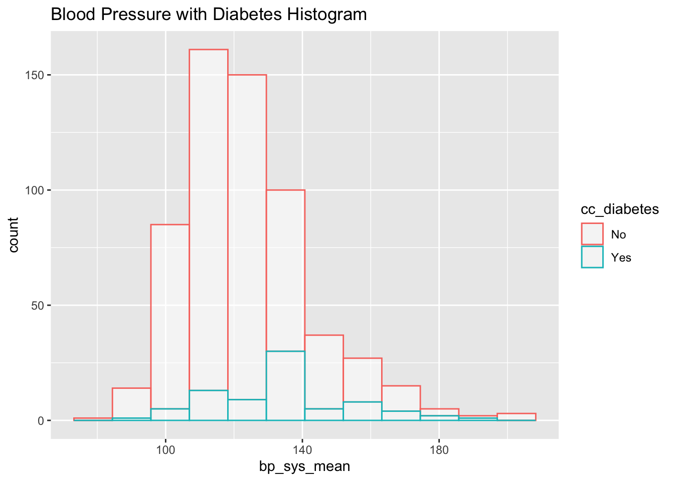

subset_nhanes%>%
  ggplot(aes(x=cc_diabetes, y=bp_sys_mean, fill=cc_diabetes)) +
    geom_boxplot() +
    scale_fill_viridis(discrete = TRUE, alpha=0.6) +
    theme_ipsum() +
    theme(
      legend.position="none",
      plot.title = element_text(size=11)
    ) +
    ggtitle("Blood Pressure VS Diabetes Status") +
    xlab("")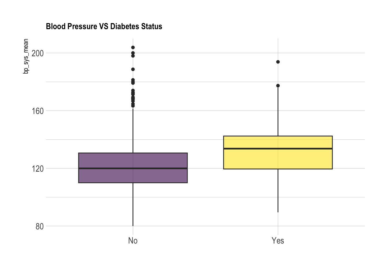

We can use a t-test to evaluate whether or not the two populations (diabetes and non-diabetes) have significantly different distributions of blood pressures:

nhanes_sys_diabetes <- subset_nhanes %>% select(cc_diabetes, bp_sys_mean) %>% drop_na(bp_sys_mean) %>% drop_na(cc_diabetes)
diabetes_test <- t.test(bp_sys_mean ~ cc_diabetes, data = subset_nhanes)
diabetes_test

    Welch Two Sample t-test

data:  bp_sys_mean by cc_diabetes
t = -5.1725, df = 97.158, p-value = 1.24e-06
alternative hypothesis: true difference in means between group No and group Yes is not equal to 0
95 percent confidence interval:
 -17.043266  -7.591128
sample estimates:
 mean in group No mean in group Yes 
         122.2213          134.5385 

Here we can see that with a p-value of 0.007, there is a significant difference between the two populations. The diabetes group has a mean blood pressure of about 137, while the non-diabetes group has a mean of about 124.

Now we want to add in noise to the data to simulate making the measurements less accurate. We can achieve this by sampling from a normal distribution centered on 0 and adding the resulting value to the original data measurement. This will mask the patient’s true blood pressure value.

We will experiment with 3 values for “reliability”: the higher the value, the lower the variance of the distribution from which we sample noise, and the closer to the original data the noisy data tends to be.

First, let’s try a value of 0.3:

    reliability <- 0.3  ### Set up measurement error with 0.5 Attenuation coef
    sigma_u_sq <- 1/reliability - 1
    
    sigma_u_sq

[1] 2.333333

    sigma_u_sq^0.5

[1] 1.527525

We can see that a low reliability value results in a variance of 2.33 and a standard deviation of about 1.53. Next, let’s increase reliability to 0.5

    reliability <- 0.5
    sigma_u_sq <- 1/reliability - 1
    
    sigma_u_sq

[1] 1

    sigma_u_sq^0.5

[1] 1

When we increase the reliability, the variance and standard deviation both decrease to 1. This will ultimately result in a bit less change to the original data.

Finally, let’s look at reliability of 0.7

    reliability <- 0.7
    sigma_u_sq <- 1/reliability - 1
    
    sigma_u_sq

[1] 0.4285714

    sigma_u_sq^0.5

[1] 0.6546537

With a variance of 0.43 and standard deviation of 0.65, this reliability value creates the least noise compared to 0.3 and 0.5.

Now, let’s actually transform the data we have and visualize:

set.seed(105)
n = nrow(subset_nhanes)

reliability <- 0.0005   ### Set up measurement error with 0.5 Attenuation coef
sigma_u_sq <- 1/reliability - 1
subset_nhanes$bp_sys_mean_noise_low <- subset_nhanes$bp_sys_mean + rnorm(n, sd=sigma_u_sq^0.5)
subset_nhanes$bp_sys_mean_noise_low <- abs(subset_nhanes$bp_sys_mean_noise_low)

reliability <- 0.005
sigma_u_sq <- 1/reliability - 1
subset_nhanes$bp_sys_mean_noise_med <- subset_nhanes$bp_sys_mean + rnorm(n, sd=sigma_u_sq^0.5)

reliability <- 0.1
sigma_u_sq <- 1/reliability - 1
subset_nhanes$bp_sys_mean_noise_high <- subset_nhanes$bp_sys_mean + rnorm(n, sd=sigma_u_sq^0.5)

Let’s visualize the difference between the raw BP measurements and the measurements with new error added in:

#X axis = Blood Pressure
#Y axis = BP + Noise
#Title = Low, Moderate, High Reliability (0.25), for example
scatterplot <- ggplot(subset_nhanes, aes(x=bp_sys_mean, y=bp_sys_mean_noise_low)) + 
    geom_point(size=0.5) +
    ggtitle("Low Reliability") +
    xlab("Blood Pressure") +
    ylab("BP + Noise")
    
scatterplot + annotate("segment", x = 75, xend = 200, y = 75, yend = 200,
  colour = "red")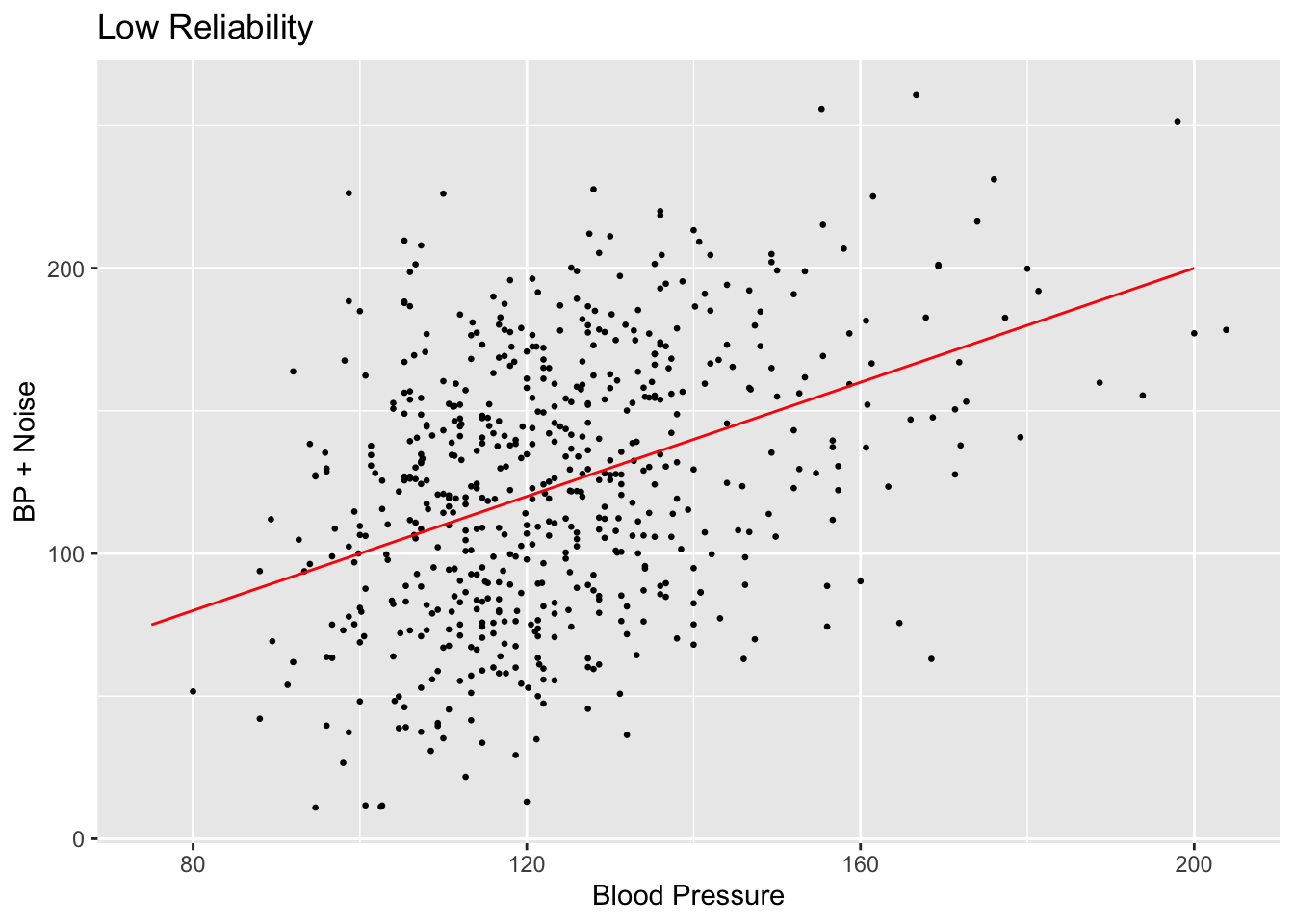

scatterplot <- ggplot(subset_nhanes, aes(x=bp_sys_mean, y=bp_sys_mean_noise_med)) + 
    geom_point(size=0.5) +
    ggtitle("Medium Reliability") +
    xlab("Blood Pressure") +
    ylab("BP + Error")
    
scatterplot + annotate("segment", x = 75, xend = 200, y = 75, yend = 200,
  colour = "red")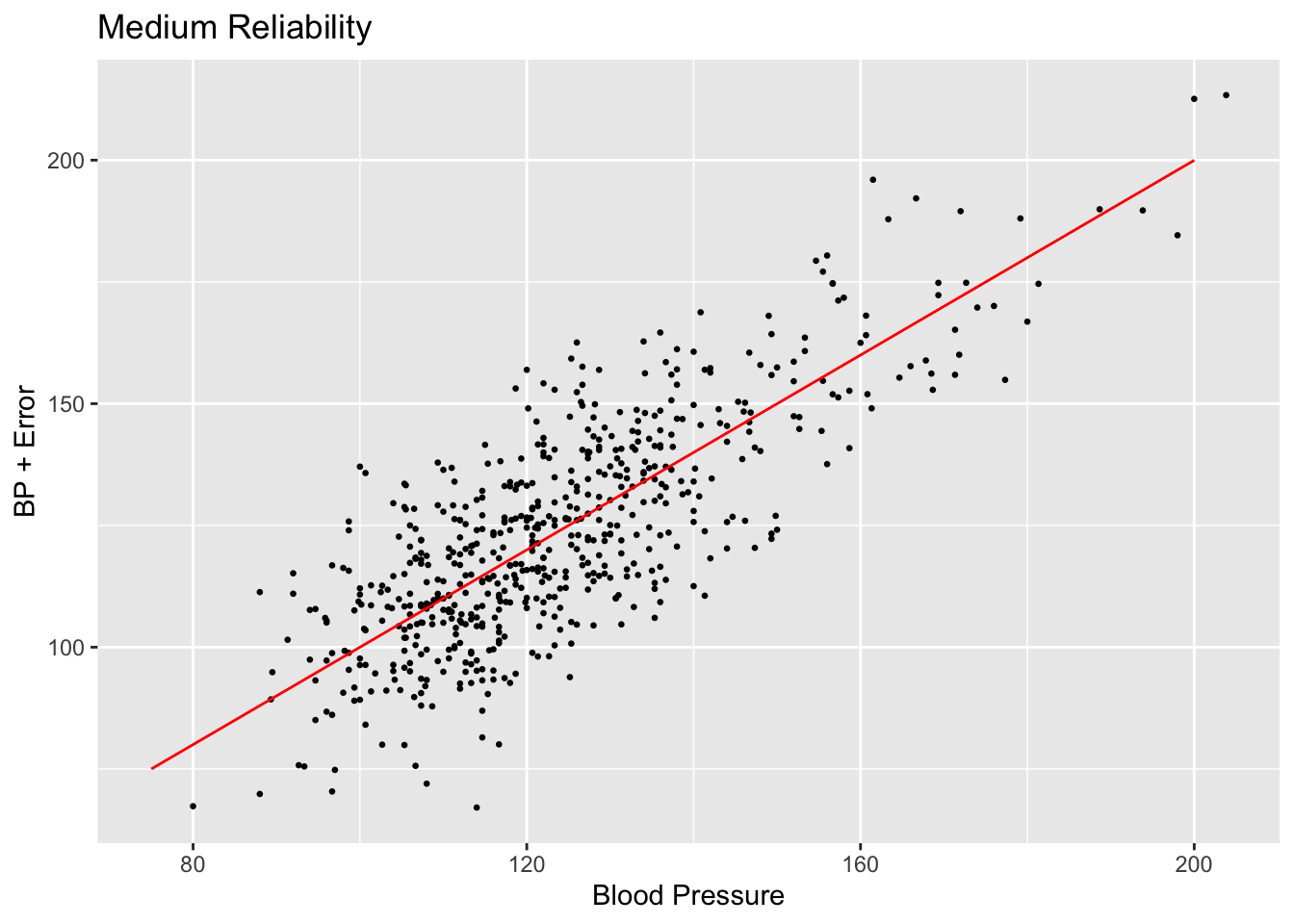

scatterplot <- ggplot(subset_nhanes, aes(x=bp_sys_mean, y=bp_sys_mean_noise_high)) + 
    geom_point(size=0.5) +
    ggtitle("High Reliability") +
    xlab("Blood Pressure") +
    ylab("BP + Error")
    
scatterplot + annotate("segment", x = 75, xend = 200, y = 75, yend = 200,
  colour = "red")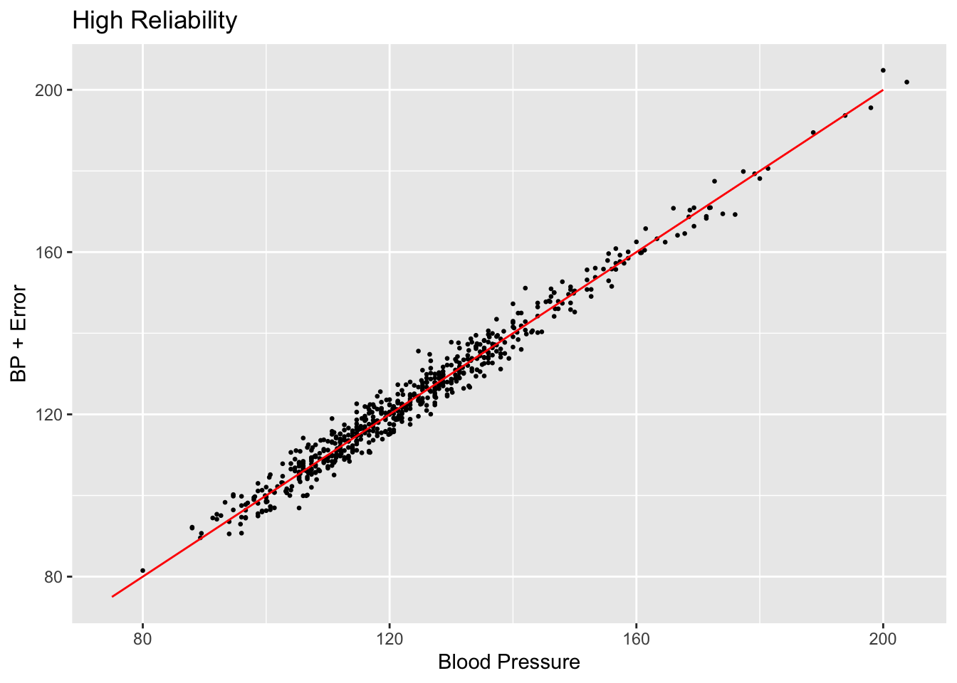

Comparing the values created by setting reliability to 0.025 and 0.25, we can see that the spread of the scatter plot is much different. The added amount of noise in the high reliability case does not shift the data points very far off from their original positions compared to the low reliability case.

We can also measure the “spread” of the noise by calculating the correlation coefficient. This will give us a numerical value for how linked the two variables are:

In some cases:

Notice that in the low reliability case, so much noise here is added that there are a few data points with a blood pressure value below 0. Data with this much error in it obviously wouldn’t be used in the real world, but for the sake of demonstrating the effectiveness of measurement error correction, we will continue to use this data.

print(paste("Reliability Low Correlation Coefficient:", cor(subset_nhanes$bp_sys_mean, subset_nhanes$bp_sys_mean_noise_low))) 

[1] "Reliability Low Correlation Coefficient: 0.371898162992643"

print(paste("Reliability Medium Correlation Coefficient:", cor(subset_nhanes$bp_sys_mean, subset_nhanes$bp_sys_mean_noise_med))) 

[1] "Reliability Medium Correlation Coefficient: 0.789073180735782"

print(paste("Reliability High Correlation Coefficient:", cor(subset_nhanes$bp_sys_mean, subset_nhanes$bp_sys_mean_noise_high)))

[1] "Reliability High Correlation Coefficient: 0.987158951684439"

Finally, let’s look again at a t-test to see if the relationship between diabetes status and noisy blood pressure is any different than the non-noisy data.

nhanes_sys_diabetes <- subset_nhanes %>% select(cc_diabetes, bp_sys_mean) %>% drop_na(bp_sys_mean) %>% drop_na(cc_diabetes)
diabetes_test <- t.test(bp_sys_mean_noise_low ~ cc_diabetes, data = subset_nhanes)
diabetes_test

    Welch Two Sample t-test

data:  bp_sys_mean_noise_low by cc_diabetes
t = -1.8332, df = 101.26, p-value = 0.06971
alternative hypothesis: true difference in means between group No and group Yes is not equal to 0
95 percent confidence interval:
 -21.4872072   0.8470414
sample estimates:
 mean in group No mean in group Yes 
         123.0366          133.3566 

nhanes_sys_diabetes <- subset_nhanes %>% select(cc_diabetes, bp_sys_mean) %>% drop_na(bp_sys_mean) %>% drop_na(cc_diabetes)
diabetes_test <- t.test(bp_sys_mean_noise_med ~ cc_diabetes, data = subset_nhanes)
diabetes_test

    Welch Two Sample t-test

data:  bp_sys_mean_noise_med by cc_diabetes
t = -4.3257, df = 105.5, p-value = 3.462e-05
alternative hypothesis: true difference in means between group No and group Yes is not equal to 0
95 percent confidence interval:
 -16.502997  -6.129374
sample estimates:
 mean in group No mean in group Yes 
         122.4257          133.7419 

nhanes_sys_diabetes <- subset_nhanes %>% select(cc_diabetes, bp_sys_mean) %>% drop_na(bp_sys_mean) %>% drop_na(cc_diabetes)
diabetes_test <- t.test(bp_sys_mean_noise_high ~ cc_diabetes, data = subset_nhanes)
diabetes_test

    Welch Two Sample t-test

data:  bp_sys_mean_noise_high by cc_diabetes
t = -5.0414, df = 96.81, p-value = 2.152e-06
alternative hypothesis: true difference in means between group No and group Yes is not equal to 0
95 percent confidence interval:
 -16.935141  -7.367393
sample estimates:
 mean in group No mean in group Yes 
         122.3786          134.5299 

We can see that in the low reliability case, enough noise was added that the results of the t-test are no longer significant, as the p-value is higher than 0.05. In the medium reliability case, the results are still significant, but much less so, with the p-value doubling from 0.02 to 0.04. Finally, in the high reliability case, the results of the t-test are not much different than when using the raw data. This is because the amount of noise added was quite low.

Now, we will try to fit a linear regression model to estimate the raw measurement from the “error”-full measurement.

error_model_0.3 <- glm(bp_sys_mean ~ bp_sys_mean_noise_low, data = subset_nhanes, family = 'gaussian')
summary(error_model_0.3)

Call:
glm(formula = bp_sys_mean ~ bp_sys_mean_noise_low, family = "gaussian", 
    data = subset_nhanes)

Coefficients:
                       Estimate Std. Error t value Pr(>|t|)    
(Intercept)           105.08228    2.04124  51.480   <2e-16 ***
bp_sys_mean_noise_low   0.15067    0.01538   9.797   <2e-16 ***
---
Signif. codes:  0 '***' 0.001 '**' 0.01 '*' 0.05 '.' 0.1 ' ' 1

(Dispersion parameter for gaussian family taken to be 304.6497)

    Null deviance: 211422  on 599  degrees of freedom
Residual deviance: 182181  on 598  degrees of freedom
AIC: 5138.2

Number of Fisher Scoring iterations: 2

error_model_0.5 <- glm(bp_sys_mean ~ bp_sys_mean_noise_med, data = subset_nhanes, family = 'gaussian')
summary(error_model_0.5)

Call:
glm(formula = bp_sys_mean ~ bp_sys_mean_noise_med, family = "gaussian", 
    data = subset_nhanes)

Coefficients:
                      Estimate Std. Error t value Pr(>|t|)    
(Intercept)           44.15721    2.57965   17.12   <2e-16 ***
bp_sys_mean_noise_med  0.64300    0.02047   31.41   <2e-16 ***
---
Signif. codes:  0 '***' 0.001 '**' 0.01 '*' 0.05 '.' 0.1 ' ' 1

(Dispersion parameter for gaussian family taken to be 133.4162)

    Null deviance: 211422  on 599  degrees of freedom
Residual deviance:  79783  on 598  degrees of freedom
AIC: 4642.8

Number of Fisher Scoring iterations: 2

error_model_0.7 <- glm(bp_sys_mean ~ bp_sys_mean_noise_high, data = subset_nhanes, family = 'gaussian')
summary(error_model_0.7)

Call:
glm(formula = bp_sys_mean ~ bp_sys_mean_noise_high, family = "gaussian", 
    data = subset_nhanes)

Coefficients:
                       Estimate Std. Error t value Pr(>|t|)    
(Intercept)              2.0698     0.8149    2.54   0.0113 *  
bp_sys_mean_noise_high   0.9822     0.0065  151.12   <2e-16 ***
---
Signif. codes:  0 '***' 0.001 '**' 0.01 '*' 0.05 '.' 0.1 ' ' 1

(Dispersion parameter for gaussian family taken to be 9.021565)

    Null deviance: 211421.9  on 599  degrees of freedom
Residual deviance:   5394.9  on 598  degrees of freedom
AIC: 3026.5

Number of Fisher Scoring iterations: 2

subset_nhanes %>%
  ggplot(aes(x=bp_sys_mean_noise_low, color=cc_diabetes)) +
    geom_histogram(fill="white", alpha=0.5, bins = 12) +
    ggtitle("Blood Pressure with Diabetes Histogram")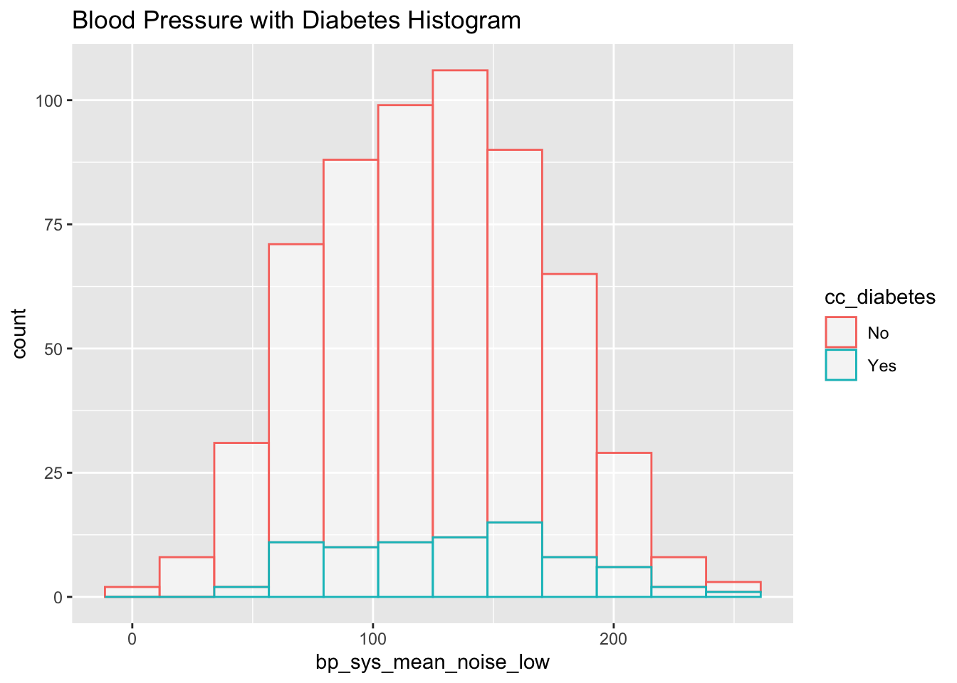

subset_nhanes %>%
  ggplot(aes(x=cc_diabetes, y=bp_sys_mean_noise_low, fill=cc_diabetes)) +
    geom_boxplot() +
    scale_fill_viridis(discrete = TRUE, alpha=0.6) +
    theme_ipsum() +
    theme(
      legend.position="none",
      plot.title = element_text(size=11)
    ) +
    ggtitle("Blood Pressure VS Diabetes Status") +
    xlab("")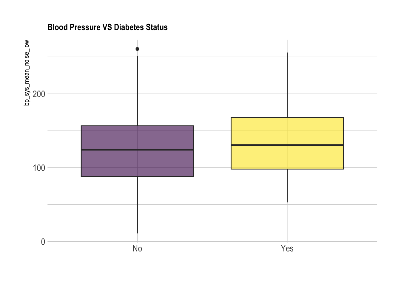

We can see in both the histogram and especially in the box plot, the noise has made it so that the two group’s distributions are virtually indistinguishable. This mimics what may happen in the real world: although the underlying distribution of two groups may be different, error in measurement may mask this fact so that the data given looks very similar. Had we been given the noisy data and performed a t-test without accounting for this error, we would come to the incorrect conclusion that diabetes and blood pressure are not linked.

This is the main issue that measurement error seeks to correct. By using it, we can avoid drawing incorrect conclusions about our data.

#Store our dataframe:
saveRDS(subset_nhanes, "nhanes_subset.rds")